
11. Discharge routing#
The FEST model can route surface runoff to compute discharge using
the Muskingum-Cunge-Todini equation [Todini, 2007], following the stream
network as delineated in morphological properties module.
Discharge routing is activated by filling the specific section
in the main configuration file ( Section 3.10 ).
This chapter describes the discharge routing configuration file,
usually named discharge-routing.ini.
Example of discharge routing configuration file.
export-channel-grid = 0

masks-number = 1

[reservoirs]
  file = ./conf/reservoirs.ini
  dt = 10
  dt-out = 3600

[diversions]
  file = ./conf/diversions.ini
  dt = 0
  dt-out = 3600

[discharge-in]
  scalar = 0.0


[discharge-out]
  scalar = 0.0

[discharge-lat]
  scalar = 0.0

[base-mask]
  channel-initiation-method = area
  channel-initiation-threshold = 4000000.
  hillslope-width = 200.
  hillslope-alpha = 45.
  hillslope-ks = 2.


Table Start
Title: channel properties
Id: base-mask
Columns:    [count]      [threshold]     [width]   [alpha]   [ks]
Units:        [-]           [m^2]          [m]      [deg]    [m^1/3s^-1]
		1            5000000           5         45        20
		2           10000000           7         45        25
		3           15000000          10         45        30
		4           20000000          20         45        35
		5           30000000          25         45        40
		6          100000000          35         45        45
		7          500000000          50         45        45
		8         1000000000          65         45        45
		9         2000000000          80         45        45
Table End
The parameters to define are listed and described in Table 11.1.
Keyword |
Description |
Requirements |
|---|---|---|
|
1 = file |
MANDATORY |
|
number of masks to assign channel parameters (at least 1 for the base-mask must exist) |
MANDATORY |
|
Section to configure reservoirs |
MANDATORY |
|
File with information about reservoirs ( Section 11.1 ) |
MANDATORY |
|
Computation time step (s) |
MANDATORY. When |
|
Time step for writing reservoirs simulation results (s). |
OPTIONAL. default value = 0. When keyword is not defined or =0, files are not written |
|
Section to configure diversions |
MANDATORY |
|
File with information about diversions ( Section 11.2 ) |
MANDATORY |
|
Computation time step (s) |
MANDATORY. When |
|
Time step for writing diversions simulation results (s). |
OPTIONAL. default value = 0. When keyword is not defined or =0, files are not written |
|
Map of input discharge initial value (m3/s) |
OPTIONAL. default value = 0. It can be set to a constant value using the |
|
Map of output discharge initial value (m3/s) |
OPTIONAL. default value = 0. It can be set to a constant value using the |
|
Map of lateral discharge initial value (m3/s) |
OPTIONAL. default value = 0. It can be set to a constant value using the |
|
Section for assigning discharge routing parameters to the entire simulation domain |
MANDATORY |
|
Method to define channel initiation. Available methods: |
MANDATORY |
|
Threshold value to initiate channel (m²) |
MANDATORY |
|
Hillslope cross section width (m) |
MANDATORY |
|
Hillslope slope of trapezoidal section side bank (degree) |
MANDATORY |
|
Hillslope Strickler roughness coefficient (m^(1/3) s⁻¹) |
MANDATORY |
A table with id = base-mask is required to define routing parameters to be used
on channel cells of the whole simulation domain. The user must include
the same parameters specified for hillslope cells (section width,
bank slope, Strickler coefficient) that can vary with basin area (m²).
The parameter values are linearly interpolated between boundary
values according to the basin area of the current cell. The [count]
column with an incremental counter is required in the table.
Different hillslope and channel parameters can be assigned to a
specific subbasin within the simulation domain. To do so, assuming
the user needs to assign parameters on N subbasins,
new sections with name [maskX] must be added, with X= 1, N.
The total number of masks (masks-number) must be updated accordingly
to account for the base-mask and the additional subbasins.
A table with id name equals to the section name (example mask1) is used
to assign channel parameters to the subbasin. In the following example,
routing parameters are assigned to the base mask and an additional subbasin.
Example of discharge routing configuration file with base-mask and the additional subbasin mask1.
masks-number = 2

[base-mask]
  channel-initiation-method = area
  channel-initiation-threshold = 4000000.
  hillslope-width = 200.
  hillslope-alpha = 45.
  hillslope-ks = 2.

[mask1]
  file = ./data/subbasin1.asc
  format = esri-ascii
  epsg = 32633
  channel-initiation-method = area
  channel-initiation-threshold = 400000.
  hillslope-width = 200.
  hillslope-alpha = 45.
  hillslope-ks = 5.

Table Start
Title: channel properties
Id: base-mask
Columns:    [count]      [threshold]     [width]   [alpha]   [ks]
Units:        [-]           [m^2]          [m]      [deg]    [m^1/3s^-1]
		1            5000000           5         45        20
		2           10000000           7         45        25
		3           15000000          10         45        30
		4           20000000          20         45        35
Table End

Table Start
Title: channel properties
Id: mask1
Columns:    [count]      [threshold]     [width]   [alpha]   [ks]
Units:        [-]           [m^2]          [m]      [deg]    [m^1/3s^-1]
		1            3000000          10         45        10
		2           12000000          15         45        15
		3           20000000          20         45        20
		4           30000000          30         45        25
		5           40000000          40         45        30

Table End
11.1. Reservoirs#
When reservoirs are activated in discharge routing configuration file, the user must provide information of reservoirs in a specific file (see example below). Two types of reservoirs are available, on-stream and off-stream reservoirs. On-stream reservoirs are the ones that are located across a river. An off-stream reservoir is a reservoir that is not located on a streambed, and is supplied by an artificial canal or pipeline. In case of off-stream reservoirs, the water stored can be released in a downstream section of the same river from which water was withdrawn, or in a different water courses.
The reservoirs configuration file contains three main keywords that configure general properties common to all reservoirs (Table 11.2).
Keyword |
Description |
Requirements |
|---|---|---|
|
Number of reservoirs to configure |
MANDATORY |
|
Epsg coordinate system id |
MANDATORY |
|
Path to file saved from a previously run simulation |
OPTIONAL |
When path-hotstart is set, initial reservoir stage and discharge
values in diversion channels, if present, are set to the resulting
values simulated in a past FeST run. In this case, past values
are read from tables written in the external file defined by path-hotstart.
Example of such a file is shown as follows.
Table Start
Title: reservoir stage at: 2020-12-07T03:00:00+00:00
Id: reservoir stage
Columns: [id] [stage]
Units: [-] [m]
1 651.7900
2 803.0000
3 803.2100
4 640.0000
…
12 747.0000
13 382.0000
14 370.0000
Table End


Table Start
Title: diverted discharge at: 2020-12-07T03:00:00+00:00
Id: diverted discharge
Columns: [id] [Qin] [Qout]
Units: [-] [m3/s] [m3/s]
1 0.3693309 8.299407
2 2.250000 2.250000
3 9.750000 9.750000
4 6.000000 6.000000
…
10 7.831643 10.37083
Table End
For each reservoir the user must configure the specific section numbered from 1 to the total number of reservoirs, filling in the required information according to the reservoir type, as listed and described in the following tables: Table 11.3, Table 11.4, Table 11.5.
Keyword |
Description |
Requirements |
|---|---|---|
|
Number Id of reservoir. Integer number from 1 to nreservoirs. |
MANDATORY. |
|
available options: on for on-stream reservoir, off for off-stream reservoir, bypass for by-pass channel. |
MANDATORY |
|
Name of the reservoir |
MANDATORY |
|
Runge-kutta integration order. Available options: 3, 4 |
MANDATORY |
|
x-coordinate of reservoir |
MANDATORY |
|
y-coordinate of reservoir |
MANDATORY |
|
Initial water surface elevation of reservoir |
MANDATORY |
|
The name of file of stage values in fest time series format that is treated as a target stage for on-stream reservoir, outlet discharge is adjusted to reach the target (on-stream type 2 reservoir) |
OPTIONAL |
|
The name of file of observed reservoir downstream discharge. The read value is used to overwrite the value computed by the FeST. The reservoir mass conservation equation does not change |
OPTIONAL |
|
The name of file of observed reservoir diverted discharge. The read value is used to overwrite the value computed by the FeST. The reservoir mass conservation equation does not change |
OPTIONAL |
|
environmental flow (m³/s), minimum value of discharge to be released from reservoir. It is used when |
Required to be used in combination with |
|
free flow discharge (m³/s). When Qin < free flow and stage <= free flow elevation Qout = Qin |
OPTIONAL. When not defined, default value = 0 |
|
free flow elevation (m asl). When Qin < free flow and stage <= free flow elevation Qout = Qin |
OPTIONAL. When not defined, default value = 0 |
|
File containing information of the stage-volume, stage-area, and stage-outlet discharge of the reservoir. See example below. |
MANDATORY |
An example of geometry file of a reservoir follows.
Column header [1] denotes the day of year since outlet discharge is valid.
When only one day (and one column) is defined, discharge is used throughout the year.
A different outlet discharge column can be set for each day of the year (doy) by
adding on column with the proper doy as header.
Example of geometry file of a reservoir
Table     Start
Title:  reservoir
Id: pusiano #   mandatory
Columns:    [h]     [area]    [volume]     [1]
Units:      [m]     [m2]       [m3]        [m3/s]
            200.0  5500000    77000000     0.0
            259.0  5500000    77000000     0.0
            260.05 5500000    77000000     10.0
            260.55 5500000    77000000     15.0
            261.0  5500000    77000000     20.0
            261.37 5500000    77000000     25.0
            261.65 5500000    77000000     30.0
            261.93 5500000    77000000     35.0
            262.17 5500000    77000000     40.0
Table   End
On-stream reservoirs may have two optional subsections, one to manage high flow condition, and the second one to include in the reservoir the simulation a channel that diverts flow from the reservoir itself (like in the example of dam for hydropower production where flow is diverted to the power production plant).
Keyword |
Description |
Requirements |
|---|---|---|
|
Marks the beginning of subsection to manage high flow condition of on-stream reservoir |
OPTIONAL. |
|
full reservoir level (m) |
MANDATORY |
|
option to manage reservoir outflow. Only option available is |
MANDATORY |
|
when |
MANDATORY |
|
Marks the beginning of subsection to manage flow diversion from reservoir |
OPTIONAL. |
|
File containing table of stream-diverted discharges relationship |
MANDATORY |
|
x-coordinate corresponding to the cell where discharge is released |
MANDATORY |
|
y-coordinate corresponding to the cell where discharge is released |
MANDATORY |
|
environmental flow (m³/s), minimum value of discharge to be released in the river downstream the diversion. To assign a changeable value during the year, a table on external file must be assigned (Section 14) |
OPTIONAL |
|
Channel length (m) |
MANDATORY |
|
Channel slope (m/m) |
MANDATORY |
|
Channel Manning roughness coefficient (s m^(-1/3)) |
MANDATORY |
|
Channel section bottom width (m) |
MANDATORY |
|
Channel section bank slope (degree) |
MANDATORY |
Example of on-stream reservoir with optional subsections for managing high flow and diversion channel
[1]
 id = 1
 type = on # on-stream reservoir
 name = santa_caterina
 rk = 4
 easting =   305461.27
 northing = 5157052.89
 stage-target-file = ./data/santa_caterina_stage.fts
 stage = 803.
 e-flow =0.852930122 # environmental flow [m3/s]
 geometry = ./data/reservoir_geometry/santa_caterina_diga.tab
[[manage-high-level]]
   full-reservoir-level = 826.2
   qout = qin
   rising = 1
[[diversion]]
   weir = ./data/reservoir_weir/diversion-weir.tab
   xout = 304514.806 # x coordinate of outflow
   yout = 5151740.539 # y coordinate of outflow
   channel-lenght = 7200 # [m]
   channel-slope = 0.017 # [m/m]
   channel-manning = 0.025 #s m^-1/3
   section-bottom-width = 10 # [m]
   section-bank-slope = 45 # [degree]
Content of diversion-weir.tab file
Table	Start
Title:	weir
Id:	G_0001-	#	mandatory
	Columns:	[Qstream]	[31]		[45]		[118]
	Units:	[m3/s]	[m3/s]	[m3/s]	[m3/s]
			0.		0.		0.		0.
			0.853		0.		0.		0.
			11.64		10.787	15.0		5.0
			10000		10.787	15.0		5.0
Table	End
Keyword |
Description |
Requirements |
|---|---|---|
|
Number Id of reservoir. Integer number |
MANDATORY. |
|
available options: on for on-stream reservoir, off for off-stream reservoir |
MANDATORY |
|
Name of the reservoir |
MANDATORY |
|
Runge-kutta integration order. Available options: 3, 4 |
MANDATORY |
|
x-coordinate of reservoir |
MANDATORY |
|
y-coordinate of reservoir |
MANDATORY |
|
Initial water surface elevation of reservoir |
MANDATORY |
|
this is the maximum stage for off-stream reservoir. When maximum stage is reached, discharge cannot enter the detention basin anymore. |
MANDATORY |
|
File containing information of the stage-volume, stage-area, and stage-outlet discharge of the reservoir. See example below. |
MANDATORY |
|
File containing information of the diverted discharge for a given discharge value in the stream |
Required when |
|
x-coordinate corresponding to the cell where discharge is released |
Required when |
|
y-coordinate corresponding to the cell where discharge is released |
Required when |
Example of weir file.
Table   Start
Title:  weir
Id: weir_csno   #   mandatory
Columns:    [Qstream]       [1]
Units:      [m3/s]           [m3/s]
              4.2              0.2
              5.1              1.3
              5.7              2.2
              6.4              3.0
              7.1              4.0
              7.8              5.0
              8.5              5.9
              9.2              6.8
              9.9              7.7
             10.6              8.5
             11.5              9.4
             12.4             10.3
             13.1             11.1
Table   End
Some examples of the different type of reservoirs that can be simulated by the FEST model are described in the following sections.
Note
Since version 1.5 of the Reservoirs module, reservoir volume is written to output file alongside water surface elevation
11.1.1. Dam and lake simulation#
Lake Idro or Eridio is a lake of glacial origin located in the province of Brescia on the border with Trentino, in Northern Italy. Situated at 368 meters above sea level, it is formed by the waters of the Chiese river which is also its outlet. Its surface is 10.9 km² and reaches a maximum depth of 122 meters.
Lake Idro is the first natural Italian lake, to have been subjected to artificial regulation. The original idea of constructing a dam dates back to 1855, but the concession was given jointly to Società Elettrica Bresciana (SEB) and the University of Naviglio Grande Bresciano in 1917 to reduce Lake Idro to a regulated reservoir, in order to produce electricity and have greater volumes of water for the summer irrigation of the Brescia and Mantua areas. The regulation work was built in the 1920s and came into operation in 1933 with a regulation which provides for a level excursion of up to 3.5 meters, later raised to 7 meters. In the period between 1950 and 1960, the company SEB (now HDE) was granted the right to build two new hydroelectric plants upstream of Lake Idro, in the Alto Chiese basin in the province of Trento, including the construction of the artificial reservoirs of Malga Bissina (1791 meters above sea level 60 million m³) and Malga Boazzo (1225 meters above sea level, 12 million m³) for a total of 72 million m³.
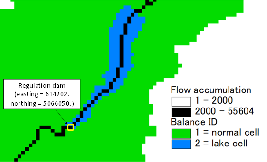
Fig. 11.1 Location of the Idro lake regulation dam along the flow accumulation map of the Chiese river basin#
The reservoirs.ini file to include the Idro lake along the Chiese river
course is shown hereafter. Coordinates of the lake match the location of the regulation dam.
nreservoirs = 1
epsg = 32632

[1]
  id = 1
  type = on
  name = idro
  rk = 4
  easting = 614202.
  northing = 5066050.
  stage = 366.0
  geometry = ./data/lake_idro.tab
The lake_idro.tab file is shown hereafter.
Table	  Start
Title:	reservoir
Id:	idro
	Columns:	[h]	    [area]	  [volume]       [1]
	Units:	 [m]	     [m2]       [m3]	      [m3/s]
     		364.00	10900000.0	1308000000.0	0.0
     		364.50	10900000.0	1313450000.0	0.0
     		365.00	10900000.0	1318900000.0	5.0
     		365.50	10900000.0	1324350000.0	10.0
     		366.00	10900000.0	1329800000.0	15.0
     		366.50	10900000.0	1335250000.0	20.0
     		367.00	10900000.0	1340700000.0	25.0
     		367.50	10900000.0	1346150000.0	30.0
     		368.00	10900000.0	1351600000.0	35.0
     		368.50	10900000.0	1357050000.0	40.0
     		369.00	10900000.0	1362500000.0	45.0
     		369.50	10900000.0	1367950000.0	50.0
     		370.00	10900000.0	1373400000.0	55.0
     		370.50	10900000.0	1378850000.0	60.0
     		371.00	10900000.0	1384300000.0	65.0
     		371.50	10900000.0	1389750000.0	70.0
     		372.00	10900000.0	1395200000.0	75.0
     		372.50	10900000.0	1400650000.0	80.0
Table	End
When the model runs produces a file that contains water elevation inside the basin, upstream discharge and downstream discharge as shown hereafter. Note that the upstream discharge, the one that enters the lake, when the lake surface is assigned the balance id = 2, may be negative when the evapotranspiration is greater than runoff. This is likely to happen at initial time steps when discharge is zero and rainfall is not occurring on the basin.
Output file.
FEST: reservoir routing
 reservoir: idro
 id:           1

 data
DateTime	  h[m]	    Qupstream[m3/s]	Qdownstream[m3/s]
2014-11-01T00:00:00+00:00     365.999      -0.001      14.991
2014-11-01T01:00:00+00:00     365.995      -0.001      14.954
2014-11-01T02:00:00+00:00     365.992      -0.001      14.918
2014-11-01T03:00:00+00:00     365.988      -0.001      14.881
…
2014-11-10T13:00:00+00:00     365.706       5.603      12.056
2014-11-10T14:00:00+00:00     365.703       7.105      12.032
2014-11-10T15:00:00+00:00     365.703      10.624      12.032
2014-11-10T16:00:00+00:00     365.703      14.249      12.032
2014-11-10T17:00:00+00:00     365.703      16.049      12.032
2014-11-10T18:00:00+00:00     365.703      16.914      12.032
2014-11-10T19:00:00+00:00     365.705      18.193      12.045
2014-11-10T20:00:00+00:00     365.708      20.989      12.082
2014-11-10T21:00:00+00:00     365.712      27.141      12.119
2014-11-10T22:00:00+00:00     365.719      38.665      12.185
2014-11-10T23:00:00+00:00     365.730      56.333      12.302
2014-11-11T00:00:00+00:00     365.747      71.968      12.473
2014-11-11T01:00:00+00:00     365.769      80.812      12.688
…
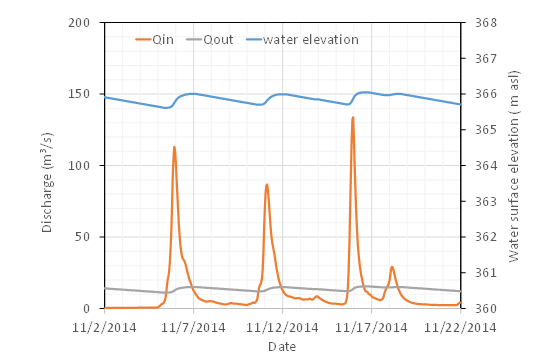
Fig. 11.2 Input and output discharge and water elevation inside the Idro lake simulated by FEST model#
11.1.2. Dam with an assigned level in time#
Malga Bissina dam is located in the Trento province (Italy), and in the Chiese river basin. It has a volume of about 61 milion m³ that is used for hydropower production. In this application the purpose is to perform a simulation following a prescribed target water level that defines the usual dam regulation. The used target water levels are not real observations, they are synthetic data generated just for demonstration purposes. When a target stage is assigned in a on-stream dam, the simulation of the water surface elevation within the basin solves the mass balance equation by setting the outflow discharge as:
When water surface is lower than target water level, outflow is computed as the minimum between the inflow discharge and the environmental flow.
When water surface is greater than target water level, outflow is computed as the maximum between the environmental flow and the value retrieved from the dam geometry table.
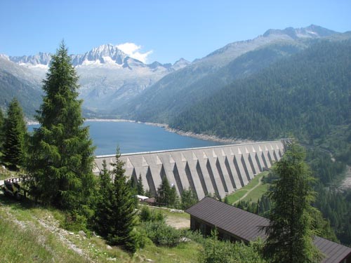
Fig. 11.3 The Malga Bissina dam on the Chiese river for hydropower production. (image source: https://dgdighe.mit.gov.it/categoria/articolo/_dighe_di_rilievo/diga_malga_bissina.#
The reservoirs.ini file to include the Malga Bissina dam is shown hereafter.
nreservoirs = 1
epsg = 32632

[1]
  id = 2
 type = on
 name = bissina
 rk = 4
 easting = 617452.
 northing = 5101300.
 stage-target-file = ./data/bissina_stage.fts
 stage = 1779.
 e-flow = 0.08 # environmental flow [m3/s]
 geometry = ./data/bissina.tab
The bissina.tab file is shown hereafter.
Table	  Start
Title:	reservoir
Id:	pusiano	#	mandatory
	Columns:	[h]	    [area]	  [volume]       [1]
	Units:	 [m]	 	 [m2]       [m3]		[m3/s]
              1740.0	762500.0	24400000.0		1.0
              1741.0	762500.0	25162500.0		1.0
              1742.0	762500.0	25925000.0		1.0
              1743.0	762500.0	26687500.0		1.0
              1744.0	762500.0	27450000.0		1.0
              …
              1775.0	762500.0	51087500.0		4.0
              1776.0	762500.0	51850000.0		5.0
              1777.0	762500.0	52612500.0		6.0
              1778.0	762500.0	53375000.0		7.0
              1779.0	762500.0	54137500.0		10.0
              1780.0	762500.0	54900000.0		15.0
              1781.0	762500.0	55662500.0		30.0
              1782.0	762500.0	56425000.0		50.0
              1783.0	762500.0	57187500.0		100.0
              1784.0	762500.0	57950000.0		313.69
              1785.0	762500.0	58712500.0		336.14
              1786.0	762500.0	59475000.0		393.57
              1787.0	762500.0	60237500.0		470.69
              1788.0	762500.0	61000000.0		563.22
              1789.0	762500.0	61762500.0		706.65
Table	End
The bissina_stage.fts file is shown hereafter.
description	=	water surface elevation
unit	=	m asl
epsg	=	32632
count	=	1
dt	=	3600
missing-data	=	-999
offsetz	=	0


metadata
Malga_Bissina_Dam	1	0	0	0

data
DateTime	1
2003-01-01T00:00:00+01:00	1782.498
2003-01-01T01:00:00+01:00	1782.498
2003-01-01T02:00:00+01:00	1782.498
2003-01-01T03:00:00+01:00	1782.498
…
2007-04-16T20-00-00+01:00	1779.516
2007-04-16T21-00-00+01:00	1779.516
2007-04-16T22-00-00+01:00	1779.516
2007-04-16T23-00-00+01:00	1779.516
2007-04-17T00-00-00+01:00	1779.486
2007-04-17T01-00-00+01:00	1779.486
2007-04-17T02-00-00+01:00	1779.486
2007-04-17T03-00-00+01:00	1779.486
2007-04-17T04-00-00+01:00	1779.486
2007-04-17T05-00-00+01:00	1779.486
2007-04-17T06-00-00+01:00	1779.486
…
When the model runs produces a file that contains water elevation inside the basin upstream discharge and downstream discharge as shown hereafter.
FEST: reservoir routing
 reservoir: bissina
 id:           2

 data
DateTime	h[m]	Qupstream[m3/s]	Qdownstream[m3/s]
2004-01-01T01:00:00+00:00    1779.000       0.000       0.000
2004-01-01T02:00:00+00:00    1779.000       0.000       0.000
2004-01-01T03:00:00+00:00    1779.000       0.000       0.000
…
2008-04-11T03:00:00+00:00    1779.574       3.675       0.020
2008-04-11T04:00:00+00:00    1779.574       3.562       0.020
2008-04-11T05:00:00+00:00    1779.574       3.197       0.020
2008-04-11T06:00:00+00:00    1779.574       2.902       0.020
2008-04-11T07:00:00+00:00    1779.574       3.572       0.020
2008-04-11T08:00:00+00:00    1779.574       8.151       0.020
2008-04-11T09:00:00+00:00    1779.575      11.380      12.873
2008-04-11T10:00:00+00:00    1779.575      10.492      12.873
2008-04-11T11:00:00+00:00    1779.574      14.306      12.872
2008-04-11T12:00:00+00:00    1779.574      12.495      12.872
2008-04-11T13:00:00+00:00    1779.575       9.716      12.874
2008-04-11T14:00:00+00:00    1779.575       8.743      12.874
2008-04-11T15:00:00+00:00    1779.575      10.809      12.874
…
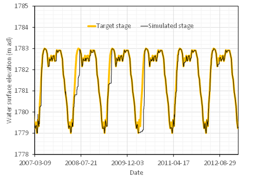
Fig. 11.4 Water surface elevation simulated by FEST model and assigned as target#
11.1.3. On stream detention basin#
The Gurone dam is an example of on stream detention basin that was put into operation in 2010 to mitigate flood risk on the Olona river, in northern Italy. The basin stores a total volume of 1.79 Mm³. Two gates regulate the basin outflow to keep the maximum discharge below 36 m³/s. When the water elevation inside the basin exceeds 289.3 m asl, water is evacuated from a 114 m length spillway with a maximum capacity of 175 m³/s at the maximum water elevation of 290.57 m asl. The minimum water level in the basin is 278.9 m asl.
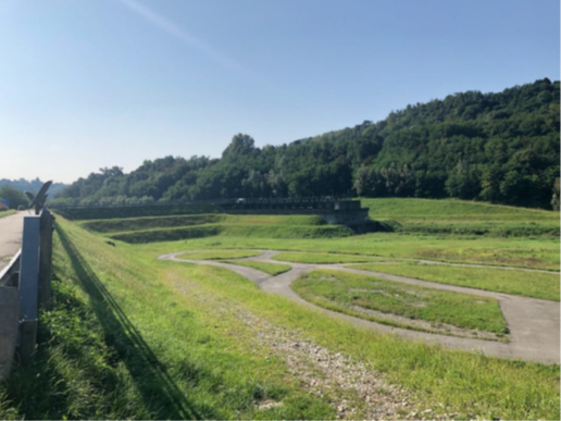
Fig. 11.5 The Gurone dam on the Olona river for flood risk mitigation. (image source: PIANO EMERGENZA DIGA – PED DIGA DI OLONA (VA).#
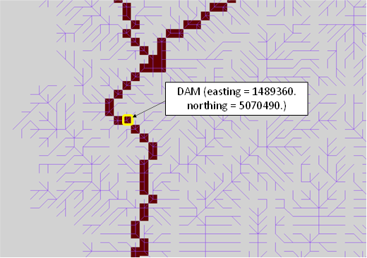
Fig. 11.6 Location of the Gurone dam along the flow accumulation map of the Olona river basin#
The reservoirs.ini file to include the Gurone detention basin along
the Olona river course is shown hereafter.
nreservoirs = 1
epsg = 3003

[1]
  id = 3
  type = on #on-stream
  name = gurone
  rk = 4 #runge-kutta order
  easting = 1489360.
  northing = 5070490.
  stage = 278.9 #initial stage [m asl]
  free-flow = 10. #[m3/s]
  free-flow-elevation = 278.9 #[m asl]
  geometry = ./data/gurone.tab
The gurone.tab file is shown hereafter.
Table	Start
Title:	reservoir
Id:	gurone
	Columns:	[h]		[area]	[volume]	[1]
	Units:	[m]		[m2]		[m3]		[m3/s]
			278.9		153385	0		0
			279.0		153385	15338.5	10
			279.1		153385	30677		15
			279.2		153385	46015.5	36
			289.3		153385	1595204	36
			290.57	153385	1790002.95	211
Table	End
When the model runs produces a file that contains water elevation inside the basin upstream discharge and downstream discharge as shown hereafter.
FEST: reservoir routing
 reservoir: gurone
 id:           3

 data
#	h[m]	Qupstream[m3/s]	Qdownstream[m3/s]
2014-11-01T00:00:00+00:00     278.900       0.000          0.000
2014-11-01T01:00:00+00:00     278.900       0.000          0.000
2014-11-01T02:00:00+00:00     278.900       0.000          0.000
…
…
2014-11-10T07:00:00+00:00     279.101      15.705         15.237
2014-11-10T08:00:00+00:00     279.111      17.758         17.256
2014-11-10T09:00:00+00:00     279.122      20.046         19.684
2014-11-10T10:00:00+00:00     279.137      23.618         22.825
2014-11-10T11:00:00+00:00     279.159      28.280         27.381
2014-11-10T12:00:00+00:00     279.184      33.519         32.584
2014-11-10T13:00:00+00:00     279.198      35.738         35.513
2014-11-10T14:00:00+00:00     279.217      37.841         36.000
2014-11-10T15:00:00+00:00     279.289      39.639         36.000
2014-11-10T16:00:00+00:00     279.380      39.258         36.000
2014-11-10T17:00:00+00:00     279.481      41.277         36.000
2014-11-10T18:00:00+00:00     279.652      44.199         36.000
…
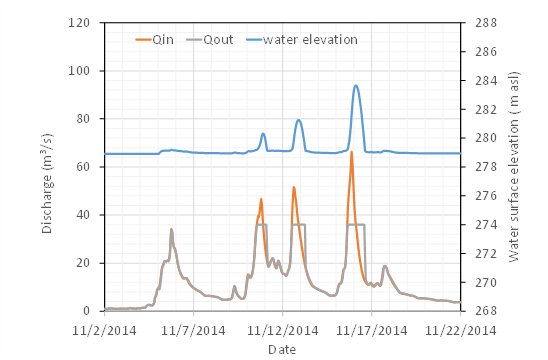
Fig. 11.7 Input and output discharge and water elevation inside the basin simulated by FEST model#
11.1.4. Dam with flow diversion#
to be completed
11.1.5. Off stream detention basin#
to be completed
11.2. Diversions#
The diversion is an hydraulic structure that diverts water from a river section to convey it to a downstream section of the same river (bypass channel) or to a different river (diversion channel).
The diversions configuration file contains two main keywords that configure general properties common to all diversions (Table below).
Keyword |
Description |
Requirements |
|---|---|---|
|
Number of diversion channels to configure |
MANDATORY |
|
Epsg coordinate system id |
MANDATORY |
|
file containing initial discharge for hotstart from a previous simulation |
OPTIONAL |
When path-hotstart is set, initial discharge values in diversion channels
are set to the results simulated in a past FeST run. In this case,
the discharge values are read from a table written in the external file
defined by path-hotstart. Example of such a file is shown as follows.
Table Start
Title: diversion status at: 2020-12-11T00:00:00+00:00
Id: diversion status
Columns: [id] [Qin] [Qout]
Units: [-] [m3/s] [m3/s]
1 0.3693309 8.299407
2 2.250000 2.250000
3 9.750000 9.750000
4 6.000000 6.000000
5 0.2000000 0.2000000
…
10 7.831643 10.37083
Table End
For each diversion the user must configure the specific section numbered from 1 to the total number of diversions, filling in the required information, as listed and described in the following table.
Keyword |
Description |
Requirements |
|---|---|---|
|
Number Id of reservoir. Integer number from 1 to nreservoirs. |
MANDATORY |
|
Name of the Name of the diversion channel |
MANDATORY |
|
x-coordinate of diversion |
MANDATORY |
|
y-coordinate of diversion |
MANDATORY |
|
File containing table of stream-diverted discharges relationship |
MANDATORY |
|
Environmental flow (m3/s), minimum value of discharge to be released in the river downstream the diversion. To assign a changeable value during the year, a table on external file must be assigned (Section 14) |
|
|
x-coordinate corresponding to the cell where discharge is released |
MANDATORY |
|
y-coordinate corresponding to the cell where discharge is released |
MANDATORY |
|
Channel length (m) |
MANDATORY |
|
Channel slope (m/m) |
MANDATORY |
|
Channel Manning roughness coefficient (s m^(-1/3)) |
MANDATORY |
|
Channel section bottom width (m) |
MANDATORY |
|
Channel section bank slope (degree) |
MANDATORY |
Some examples of diversion channels that can be simulated by the FeST model are described in the following sections.
11.2.1. Diversion channel#
The Seveso river, in Northern Italy, is a small river that flows into Milan. This area is frequently hit by high rainfall intensity events that cause severe floods. The urban development after the second World War, has reduced the river basin soil infiltration capacity and exacerbated the flood occurrences. In 1980 the canale scolmatore di nord ovest (CSNO) bypass channel was put into operation to mitigate the flood risk in Milan. It is a 34 km length channel that deviates a maximum discharge of 30 m³/s from the Seveso river to convey it into the Ticino river.
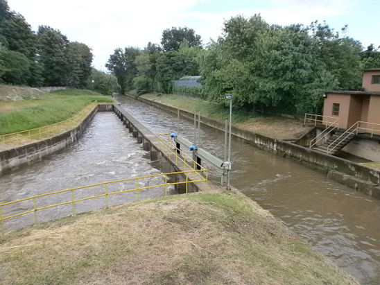
Fig. 11.8 The CSNO bypass channel on the Seveso river. Source: Stefano Stabile, CC BY-SA 3.0 <https://creativecommons.org/licenses/by-sa/3.0\>, via Wikimedia Commons#
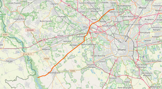
Fig. 11.9 Path of the CSNO bypass channel. Source: https://www.openstreetmap.org/relation/4633456#
The diversions.ini file to include the CSNO diversion channel along the
Seveso river is shown hereafter. Note that xout and yout are set to
0 because the outlet section of the diversion channel is outside the simulation domain.
ndiversions = 1
epsg = 3003

[1]
 id = 2
 name = csno
 easting = 1512560.
 northing  = 5047490.
 weir = ./data/weir_csno.tab
 xout = 0 # x coordinate of outflow
 yout = 0 # y coordinate of outflow
 channel-lenght = 34000 # [m]
 channel-slope = 0.001 # [m/m]
 channel-manning = 0.0222 #s m^-1/3
 section-bottom-width = 10. # [m]
The weir_csno.tab file is shown hereafter. Note that there is one column associated to doy 1.
The column header name is the doy itself. A column with different discharge can be assigned for each day of the year.
Table	Start
Title:	weir
Id:	weir_csno	#	mandatory
Columns:	[Qstream]	[1]
Units:		[m3/s]		[m3/s]
		0.0		0.0
		4.2		0.2
		5.1		1.3
		5.7		2.2
		6.4		3.0
		7.1		4.0
		7.8		5.0
		8.5		5.9
		9.2		6.8
		9.9		7.7
		10.6		8.5
		…		…
		…		…
		138.0		30.1
		139.9		30.1
		141.8		30.1
		143.8		30.1
		145.7		30.1
		147.7		30.1
		149.6		30.1
Table	End
When the model runs produces a file that contains upstream and downstream discharge and input and output discharge in and from the diversion channel as shown hereafter.
FEST: diversion routing
diversion name: csno
diversion id:           2

 data
DateTime Qupstream[m3/s]	Qdownstream[m3/s] QinChannel[m3/s]  QoutChannel[m3/s]
2014-11-01T00:00:00+00:00      0.000      0.000    0.000    0.000
2014-11-01T01:00:00+00:00      0.000      0.000    0.000    0.000
2014-11-01T02:00:00+00:00      0.000      0.000    0.000    0.000
…
2014-11-15T13:00:00+00:00     11.319      2.100    9.219    0.054
2014-11-15T14:00:00+00:00     14.208      2.100   12.108    0.376
2014-11-15T15:00:00+00:00     18.267      2.087   16.180    0.949
2014-11-15T16:00:00+00:00     22.833      2.104   20.729    2.701
2014-11-15T17:00:00+00:00     28.560      2.781   25.779    5.741
2014-11-15T18:00:00+00:00     35.337      6.279   29.057   11.028
2014-11-15T19:00:00+00:00     40.972     10.872   30.100   17.341
2014-11-15T20:00:00+00:00     44.818     14.718   30.100   22.241
2014-11-15T21:00:00+00:00     45.403     15.303   30.100   25.306
…
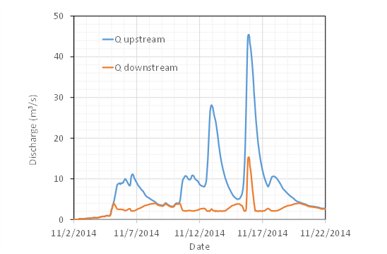
Fig. 11.10 Discharge in the Seveso river upstream and downstream the diversion channel intake section#
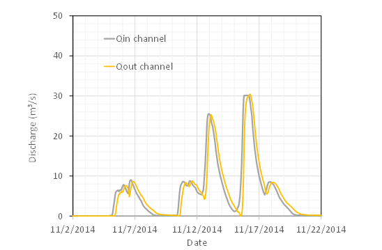
Fig. 11.11 Input and output discharge in and from the CSNO diversion channel#