
10. Soil water balance#
The soil water balance module is aimed at computing the water (and energy fluxes, optionally) and updating the soil water content. It is activated by filling the specific section in the main configuration file ( Section 3.9 ). This chapter describes the soil water balance configuration file.
Example of soil water balance configuration file.
threshold-storm-start = 1.
interstorm = 10.
infiltration = ./conf/infiltration.ini
evapotranspiration = ./conf/evapotranspiration.ini

[balance-id]
  file = ./data/balance_id.asc
  format = esri-ascii
  epsg = 3003

[soil-depth]
  file = ./data/sd.asc
  format = esri-ascii
  epsg = 3003

[root-zone-depth]
  scalar = 0.1

[ksat-subsurface]
  file = ./data/kprof.asc
  format = esri-ascii
  epsg = 3003

[deep-percolation-factor]
  scalar = 0.1

################################
# state variables initialization
################################

[saturation-rz]
  scalar = 0.3

[saturation-tz]
  scalar = 0.3
The parameters to set are listed and described in Table 10.1. For setting state variables initial value see ( Section 10.2 )
Keyword |
Description |
Requirements |
|---|---|---|
|
threshold to consider storm initiated [mm/h] |
MANDATORY |
|
duration of interstorm period to terminate an event [h] |
MANDATORY |
|
Name of file to configure infiltration simulation. See 10.3 |
MANDATORY |
|
Name of file to configure infiltration simulation. See 10.4. |
MANDATORY |
|
Map of saturated conductivity used to compute lateral subsurface flux (m/s) |
MANDATORY. It can be set with |
|
Map of balance id. 1=normal cell (hillslopes or channel); 2=lake; 3=landplain. See 10.1 for details. |
MANDATORY. |
|
Map of total soil depth (m) |
MANDATORY. It can be set with |
|
Map of root zone depth (m) |
MANDATORY. It can be set with |
|
Map of deep percolation factor, used as a limiter of deep percolation from transmission zone (-) |
OPTIONAL. It can be be set with scalar keyword. Default value = 1. |
10.1. Balance id#
Specific scheme for solving soil balance is applied according to balance id:
Id = 1, denotes hillslope and channel (normal) cells. Vertical and lateral flows are computed and used for updating soil moisture. When id = 1 cell bounds a id=3 cell lateral flow is passed to id = 3 cell as boundary flux condition (Neumann type boundary condition).
Id = 2, denotes lake cells. Soil moisture is set to saturated content, evaporation is set to potential, runoff is computed as precipitation – evaporation (negative values can occur), percolation is null.
Id = 3 denotes landplain cells that may interact with groundwater at the bottom boundary. Lateral fluxes are null, capillary rise is computed and used for updating soil moisture. Percolation is computed and passed as source term of the underlying groundwater.
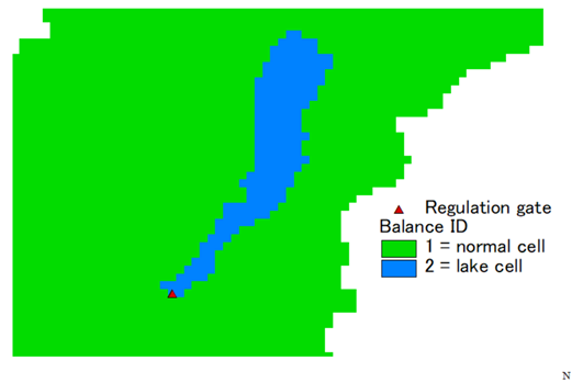
Fig. 10.1 Example of Balance id map for the simulation of the Idro lake basin, in Italy. Blue cells mark lake cells. Note the location of gate that regulates outflow and lake water surface elevation.#
10.2. State variables initialization#
State variables must be initialized when simulation starts.
Initial state can be set to an arbitrary value or to a value
saved from a previous simulation run.
It is mandatory to initialize two variables: root zone soil
saturation degree ( [saturation-rz] ), and transmission
zone soil saturation degree ( [saturation-tz] ),
either by setting a constant value ( set with scalar keyword)
or a map saved from a previous simulation run.
The actual soil water content in each cell, both in root
and transmission zones, is computed by the model according
to the soil hydrological properties of the given cell.
Two state variables can be optionally set to
an initial value: [precipitation-status] and [interstorm-duration].
Other optional state variables are required by different
infiltration models (see Table 10.2). When an optional
state variable is not assigned an initial value in the
configuration file, the default value, 0, is assigned.
A constant value can be set with scalar keyword.
Keyword |
Description |
Requirements |
|---|---|---|
|
Root zone soil saturation degree |
MANDATORY |
|
Transmission zone soil saturation degree |
MANDATORY |
|
Precipitation status. Defines if in storm or interstorm period. |
OPTIONAL |
|
Interstorm duration [mm]. Defines time from the end of the last precipitation event. |
OPTIONAL |
|
Cumulative precipitation [mm] |
OPTIONAL. Used by SCS-CN model |
|
Actual soil retention capacity at the beginning of precipitation [mm]. |
OPTIONAL. Used by SCS-CN model |
|
Cumulative infiltration [mm] |
OPTIONAL. Used by Philips and Green-Ampt infiltration models |
10.3. Infiltration#
Infiltration is defined as the water movement from the ground surface into the soil. Different infiltration equations have been implemented in the FEST model. It’s up to the user to select the equation that he desires to use depending on required outputs and available inputs. The available infiltration models are as follows:
SCS-modified curve number (SCS-CN): according to the Soil Conservation Service (SCS) (1985) modified for continuous simulation [Ravazzani et al., 2015]
Philip: according to Philip numerical solution [Philip, 1957]
Green and Ampt_according to Green and Ampt solution [Green and Ampt, 1911]
Ross-Brooks and Corey: solved according to [Ross, 2003] fast and non-iterative solution for Richard equation using water retention curve parameters according to Brooks and Corey equation [Brooks and Corey, 1966]
Ross-Van Genuchten solved according to [Ross, 2003] fast and non-iterative solution for Richard equation using water retention curve parameters according to van Genuchten equation [Van Genuchten, 1980]
Keywords in the infiltration configuration file (usually named infiltration.ini) are listed and described in Table 10.3.
Keyword |
Description |
Requirements |
|---|---|---|
|
Infiltration model to be selected by the user: 1=SCS-CN, 2=Philip, 3=Green-Ampt, 4=Ross Brooks and Corey, 5=Ross Van Genuchten. |
The user should check the available soil data before the selection of the infiltration model to be used for the simulations |
|
Soil parameters could be assigned from single file for each parameter (method number 1) or soil parameters could be assigned from soil type map (method number 2) |
For method 1 the user should provide a map for each required soil parameter, depending on the selected model. For method 2, the user should provide soil data input parameters in soil-types file. |
|
Soil type file used when parameter-assigning-method = 2 |
This keyword is mandatory if parameter assigning method = 2 |
|
Number of the subdivisions of the soil layer |
Required by Ross-Brooks and Corey, and Ross Van Genuchten models. |
|
Refers to the maximum change in the effective saturation (S), of any unsaturated layer to aim for each time step, controls time step size. This parameter is used by Ross model. |
Required by Ross-Brooks and Corey, and Ross Van Genuchten models. If not specified a default value of 0.05 is used. |
|
Refers to the bottom boundary condition for water; “free drainage” (means zero gradient of matric head),, “seepage”, or “zero flux”. |
Required by Ross-Brooks and Corey, and Ross Van Genuchten models |
|
Map of soil type |
this section is mandatory if parameter-assigning-method = 2 |
|
Map of soil hydraulic conductivity at saturation (m/s) |
Required by all infiltration models |
|
Map of residual water content (m³/m³) |
Required by all infiltration models |
|
Map of water content at saturation (m³/m³) |
Required by all infiltration models |
|
Map of field capacity (m³/m³) |
Required by all infiltration models |
|
Map of wilting point (m³/m³) |
Required by all infiltration models |
|
Map of pore size distribution index of Brooks and Corey (-) |
Required by all infiltration models |
|
Map of bubbling pressure (m) |
Required by all infiltration models |
|
Map of curve number (-) |
Required by SCS-CN |
|
Map of abstraction ratio to compute initial loss (-). Standard value = 0.2 |
Required by SCS-CN |
|
Map of curve number storativity (S₀) (mm). Standard value = 254 |
Required by SCS-CN |
|
Map of front suction head (m) |
Required by Green-Ampt |
|
Map of n shape coefficient of Van Genuchten retention curve (-) |
Required by Ross Van Genuchten |
|
Map of m shape coefficient of Van Genuchten retention curve (-) |
Required by Ross Van Genuchten |
|
Map of pore tortuosity index (-) |
Required by Ross Van Genuchten |
|
Map of conductivity at saturation of soil matrix (m/s) |
Required by Ross Van Genuchten |
In the next example, the user selected Philip equation for the simulation of the
infiltration which corresponds to the method number 2. For the determination of the
soil parameter the user selected the method 1 that implies assigning the soil
parameters from single file for each required parameter. A scale_factor is
applied to soil conductivity in order to convert the input map from cm/h to m/s unit.
model = 2 # Philip infiltration model

parameter-assigning-method = 1 # 1 = read each parameter from single file; 2 = assign parameter from soil type map

# this keyword is mandatory if parameter-assigning-method = 2
soil-types-file = ./conf/soil-types.ini

ross-divisions = 1 # number of subdivisions of soil layer

# max change in S (the "effective saturation") of any unsaturated
# layer to aim for each time step; controls time step size
# If not specified default value used = 0.05
# used by Ross model
ross-dSmax = 0.05

#initial pond depth [m] if not given default to zero
# used by Ross model
ross-hpondzero = 0.

# used by Ross model
ross-botbc = free drainage
#botbc = zero flux
#botbc = seepage

# alternative to assign soil type map is assigning single map for each parameter
[conductivity]
  file = ./dati/toce_kscmh.asc
  format = esri-ascii
  epsg = 23032
  scale_factor = 0.0000027777

[residual-water-content]
  file = ./dati/toce_tr_200.asc
  format = esri-ascii
  epsg = 23032

[saturated-water-content]
  file = ./dati/toce_ts_200.asc
  format = esri-ascii
  epsg = 23032

[field-capacity]
  file = ./dati/toce_fc_200.asc
  format = esri-ascii
  epsg = 23032

[wilting-point]
  file = ./dati/toce_wp_200.asc
  format = esri-ascii
  epsg = 23032

[pore-size-index]
  file = ./dati/toce_bc_200.asc
  format = esri-ascii
  epsg = 23032

[bubble-pressure]
  file = ./dati/toce_bp_200.asc
  format = esri-ascii
  epsg = 23032
In case the user sets parameter-assigning-method = 2 the file assigned by soil-types-file
must be prepared together with map assigned by [soil-type-map] section in the
infiltration configuration file. The list of parameters to be included in this
files depends on the selected infiltration model previously chosen. These parameters are reported in Table 10.4.
Soil parameter |
Definition |
Unit |
Model |
|---|---|---|---|
|
Saturated hydraulic conductivity |
m/s |
all |
|
saturated volumetric water content |
m3/m3 |
all |
|
residual volumetric water content |
m3/m3 |
all |
|
Water content at field capacity |
m3/m3 |
all |
|
Water content at wilting point |
m3/m3 |
all |
|
maximum soil storage |
m |
all |
|
pore-size distribution index |
- |
all |
|
Curve number |
- |
Curve Number |
|
abstraction-ratio, default value=0.2 |
- |
Curve Number |
|
Storativity |
mm |
Curve Number |
|
air entry value, bubbling pressure |
m |
Philips, ROSS-BC and ROSS-VG |
|
Suction head at the wetting front |
m |
Green and Ampt |
|
vG retention function shape parameter |
- |
ROSS-VG |
|
vG retention function shape parameter |
- |
ROSS-VG |
|
tortuosity index |
- |
ROSS-VG |
|
saturated conductivity of soil “matrix” (m/s). Different from ksat when macropores impact |
ROSS-VG |
The example below reports all parameters required by the Philips equation. The number of the soil types for the following example has been set to 2. So, the user in this case should include two sets of soil parameters.
Example of file defined by soil-types-file.
soil-types = 2

[1] # soil type number 1
  ksat = 1.74E-05   #saturated conductivity (m/s)
  thetas =  0.462  #saturated volumetric water content (m3/m3)
  thetar =  0.01  #residual volumetric water content (m3/m3)
  psdi   =  0.288 #brooks and corey pore size distribution index (-)
  psic  = 0.00452 # air entry value, bubbling pressure (m)
  wp = 0.079  # wilting point (m3/m3)
  fc = 0.278 # field capacity (m3/m3)
  smax = 0.2 # maximum soil storage (m)

[2] # soil type number 2
  ksat = 5.48E-06   #saturated conductivity (m/s)
  thetas =  0.434  #saturated volumetric water content (m3/m3)
  thetar =  0.01  #residual volumetric water content (m3/m3)
  psdi   =  0.248 #brooks and corey pore size distribution index (-)
  psic  = 0.00488 # air entry value, bubbling pressure (m)
  wp = 0.0611  # wilting point (m3/m3)
  fc = 0.297 # field capacity (m3/m3)
  smax = 0.2 # maximum soil storage (m)
10.4. Evapotranspiration#
Different equations have been implemented in the FEST model for computing evapotranspiration. The available models are as follows:
Penman-Monteith [Allen et al., 1998];
Priestley and Taylor [Priestley and Taylor, 1972] ;
Hargreaves and Samani [Hargreaves and Samani, 1982] ;
Hargreaves and Samani modified with elevation correction [Ravazzani et al., 2012];
FAO-56 Penman-Monteith [Allen et al., 1998];
Energy balance. (To be implemented in the new code)
Keywords in the evapotranspiration configuration file (usually named evapotranspiration.ini) are listed and described in Table 10.5.
Keyword |
Description |
Requirements |
|---|---|---|
|
1 = one method for the entire domain, 2 = a map with model codes |
Mandatory |
|
Evapotranspiration model: 1=Penman-Monteith, 2=Priestley-Taylor, 3=Hargreaves-Samani, 4= Hargreaves-Samani modified, 5=FAO-56 Penman-Monteith., 6=energy-balance |
Required when |
|
Computation time step (s) |
Mandatory |
|
0 = no, 1 = yes. |
Optional. If not specified crop coefficient is not applied. |
|
map of model id (see model) |
Required when |
When use-crop-coefficient = 1 the user must configure how to assign crop coefficient
values in section [crop-coefficient] Table 10.6. Crop coefficient values can be assigned in two ways:
A map of ids and a related file with crop coefficient time series value for each id in the map. When a new value of crop coefficient is read from file, the value is assigned to all cells with the same id in the map.
A time variable map encoded in Net-CDF format.
Keyword |
Description |
Requirements |
|---|---|---|
|
Section to configure crop coefficient use. |
Required when |
|
Sub-keyword in section [crop-coefficient] to define file with crop coefficient values in fest time series format or net-Cdf. |
mandatory |
|
1 = use code-map, 0 = use netcdf grid data |
mandatory |
|
1 = use code-map, 0 = use netcdf grid data |
Required when |
|
Subsection that defines the map with id code |
Required when |
In the next example, the modified Hargreaves Samani model (model = 4) is used to
compute evapotranspiration on the entire domain (model-assignment = 1) at daily
time scale (dt = 86400). Crop coefficient values are defined by reading values
from ./meteo/kc.txt (see below) file and assigned to the corresponding code in ./dati/toce_kc_code.asc map.
Example of evapotranspiration configuration file.
dt = 86400 # time step computation (s)

model-assignment = 1 # one method for the entire domain

model = 4 # modified Hargreaves model

use-crop-coefficient = 1 # 0 = no, 1 = yes

[crop-coefficient]
   file = ./meteo/kc.txt #file containing crop coefficient
   interpolation = 1  # 1 = use code-map
   [[code-map]]
     file = ./dati/toce_kc_code.asc
     format = esri-ascii
     epsg = 23032
Example of file in fest time series format with crop coefficient value to assign to id map.
description	=	crop coefficient
unit	=	-
epsg	=	23032
count	=	2
dt	=	3600
missing-data	=	-999.9
offsetz	=	0

metadata
code1	1	0	0	0
code2	2	0	0	0

data
date&time	code1	code2
2000-01-01T00:00:00+01:00	0.26	1.05
2000-01-01T01:00:00+01:00	0.26	1.05
2000-01-01T02:00:00+01:00	0.26	1.05
2000-01-01T03:00:00+01:00	0.26	1.05
2000-01-01T04:00:00+01:00	0.26	1.05
2000-01-01T05:00:00+01:00	0.26	1.05
2000-01-01T06:00:00+01:00	0.26	1.05
2000-01-01T07:00:00+01:00	0.26	1.05
2000-01-01T08:00:00+01:00	0.26	1.05
2000-01-01T09:00:00+01:00	0.26	1.05
2000-01-01T10:00:00+01:00	0.26	1.05
2000-01-01T11:00:00+01:00	0.26	1.05
...