12. Groundwater

The FEST model can simulate groundwater flow with a quasi 3D scheme based on macroscopic cellular automata [Ravazzani et al., 2011].
Groundwater is simulated as one or more aquifers that can interact through an aquitard. Aquitard depth is computed as the difference between bottom of upper aquifer and top of lower aquifer. Aquifers are enumerated starting from number 1 at top. At least one aquifer must be present in order to simulate groundwater. Optionally, the mutual flux exchange between river and groundwater can be simulated.

Groundwater simulation is activated by filling in the specific section in the main configuration file ( Section 3.11 ). This chapter describes the groundwater configuration file, usually named groundwater.ini. Aquifers configuration is explained in Table 12.1, river-groundwater interaction is explained in Table 12.2

Table 12.1 How to configure aquifers to simulate groundwater

Keyword	Description	Requirements
aquifers	Number of aquifers in the groundwater basin	Mandatory
[aquifer_n]	Section that configure the aquifer number n with n = 1, aquifers.	Mandatory
[[boundary-condition-id]]	Map of boundary condition and active cells definition. Available options: 1 = active cell, 2 = Dirichlet type boundary condition (assigned head), 3 = Neumann type boundary condition (flux assigned)	Mandatory. The user can set a map with usual file, format, and epsg keywords, or he can assign a constant value using the scalar keyword
[[boundary-condition-value]]	Map of boundary condition head values to be assigned to cells of Dirichlet type boundary condition (id = 2). For Neumann type boundary condition cells (id = 3), a flux is assigned internally at every time step from the soil water balance module.	Mandatory. The user can set a map with usual file, format, and epsg keywords, or he can assign a constant value using the scalar keyword. This map can change in time by assigning a netCDF multitemporal layer. In this case the user can set sync-initial-time = 1 option to synchronize the simulation to the proper initial map
[[top-elevation]]	Top of the aquifer.	Mandatory. The user can set a map with usual file, format, and epsg keywords, or he can assign a constant value using the scalar keyword
[[bottom-elevation]]	Bottom of the aquifer	Mandatory. The user can set a map with usual file, format, and epsg keywords, or he can assign a constant value using the scalar keyword
[[hydraulic-conductivity]]	Aquifer hydraulic conductivity (m/s)	Mandatory. The user can set a map with usual file, format, and epsg keywords, or he can assign a constant value using the scalar keyword
[[specific-yield]]	Aquifer specific yield (m/m)	Mandatory. The user can set a map with usual file, format, and epsg keywords, or he can assign a constant value using the scalar keyword
[[aquitard-conductivity]]	Aquitard hydraulic conductivity (m/s)	Required when more than one aquifer are simulated. The last (lower) aquifer does not need aquitard definition. The user can set a map with usual file, format, and epsg keywords, or he can assign a constant value using the scalar keyword

In the next example, one aquifer is configured. boundary-condition-id, initial-head, and top-elevation, are assigned as raster esri ascii maps. bottom-elevation, hydraulic-conductivity, and specific-yield, are assigned as a scalar constant. boundary-condition-value is assigned as a multitemporal net-cdf file with option sync-initial-time = 1 to start from the proper initial value.

Example of groundwater configuration file.

aquifers = 1

[aquifer_1]
   [[boundary-condition-id]]
     file = ./data/aquifer1_bc_id.asc
     format = esri-ascii
     epsg = 32632
   [[boundary-condition-value]]
     file = ./data/head_bc.nc
     format = net-cdf
     variable = head
     epsg = 32632
     sync-initial-time = 1
   [[initial-head]]
     file = ./data/dem-3m.asc
     format = esri-ascii
     epsg = 32632
   [[top-elevation]]
     file = ./data/dem.asc
     format = esri-ascii
     epsg = 32632
   [[bottom-elevation]]
     scalar = 50.
   [[hydraulic-conductivity]]
     scalar = 0.0003
   [[specific-yield]]
     scalar = 0.3

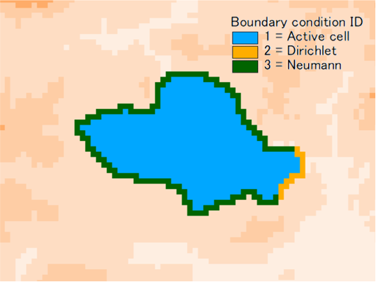
Fig. 12.1 Example of map to set boundary condition and active cell

12.1. River-groundwater flux exchange

Table 12.2 How to configure flux exchange between river and groundwater

Keyword	Description	Requirements
[river-groundwater]	It starts section to configure river-groundwater interaction	Optional
[[river-id]]	Map that defines the cells where river-groundwater interaction is simulated. 1=river-groundwater interaction cell, nodata = no interaction.	Mandatory.
[[river-dem]]	Map that specifies the river thalweg elevation. It may be different from digital elevation model assigned in Morphological properties section.	Mandatory

A table with id = river-groundwater is required to define riverbed conductivity and thickness. In the following example two maps are assigned as [[river-id]] and [[river-dem]]. Table river-groundwater defines two ids with 0.0001 and 0.0003 m/s streambed conductivity, respectively and a streambed thichness of 1 m. [[river-id]] map is shown in Fig. 12.2

Example of [river-groundwater] section in groundwater configuration file.

[river-groundwater]
  [[river-id]]
    file = ./data/river_aquifer_id.asc
    format = esri-ascii
    epsg = 32632
	
  [[river-dem]]
    file = ./data/dem-5.asc
    format = esri-ascii
    epsg = 32632
	
Table Start
Title: river groundwater exchange parameters
Id: river-groundwater

Columns: [id]   [streambed-conductivity]  [streambed-thickness]
Units:   [-]          [m/s]                      [m]            
          1          0.0001                      1.0
          2          0.0003                      1.0
Table End   

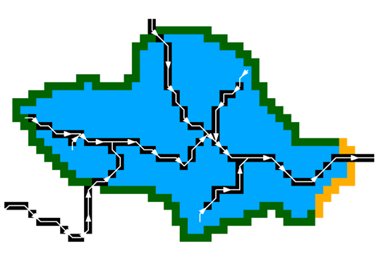
Fig. 12.2 Map of flow accumulation (black cells) and river direction (white arrow) overlayed to boundary condition id map of Fig. 12.1

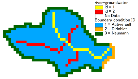
Fig. 12.3 Map of flow river-groundwater id overlayed to boundary condition id map of Fig. 12.1