5. Glacier accumulation and ablation

Glaciers are known to have a significant impact on stream flow runoff: they store water during winter season, while, during summer, melt water may provide the only source of water for some Alpine valley; they therefore play an important role on the river flow regimes with peaks of melting during the middle-late summer (Hock, 2003; Hock et al., 2005; Milner et al., 2009). The structure and space-time dynamic of a glacier is very complex; for this reason, representing in a rigorous manner the glacier dynamic within an hydrological model requires numerous input data and onerous computational time, which makes it difficult to apply to complex and extended drainage basins (Huss et al., 2008).

Several approaches exist to model glacier dynamic within hydrological models, as well as different methods exist to simulate melt and accumulation of ice. Ice melt models can be grouped in two main categories: the energy balance models and the temperature-index models (Hock, 2003); the first type of models has a strong physical basis because each of the relevant energy fluxes at the glacier surface is computed using direct measurement of meteorological variables and thus allows to obtain melt rates with high precision and with high temporal resolution; in the second type of models melt rate is calculated from empirical formulas. However, despite the simplicity of the temperature-index models, they are commonly used because of the wide availability of temperature data and the lower computational cost; furthermore, Hock (Hock, 2003) highlighted the physical basis of such kind of models. In more detailed models, accumulation is modelled taking into account snow, firn, and ice and the spatial redistribution of snow due to drift and avalanches (Huss et al., 2008); in conceptual models, accumulation of ice is not often taken into account because they typically starts from an infinite volume of ice or consider glaciers area constant in time (Klock et al., 2001); otherwise, they simply solve the mass balance between solid precipitation, snow melt and glacier melt (Schaefli et al., 2005; Horton et al., 2006; Konz and Seibert, 2010).

The glaciers module implemented within the FeST model is aimed at simulating the contribution of glacier melt to runoff for middle-size to large basins. The glaciers module is simple in structure but without losing the raster based approach of the whole model. The glacier model requires few input data (glaciers area, DEM, temperature, and precipitation) and is able to reproduce melting, with a simple temperature index melt model, accumulation and propagation of melt water into ice, in a way similar to snow simulation (see Section 4).

The module assumes that glaciers form a layer between the ground, below, and snowpack, above. When a snowpack layer is present above glacier, it protects ice from ablation and intercepts rainfall. When glacier is free from snow, the ice melt rate in m/s, \(M_{ice}\), is proportional to the difference between air temperature, \(T_{a}\) , and a predefined threshold temperature, \(T_{b,ice}\):

(5.1)\[\begin{split}M_{ice} = \left\{ \begin{aligned} & C_{m,ice}(T_{a} - T_{b,ice})\quad\mspace{6mu} if\quad T_{a} > T_{b,ice} \\ & 0\quad\quad\quad\quad\mspace{6mu} if\quad T_{a} \leq T_{b,ice} \\ \end{aligned} \right.\ \end{split}\]

where \(C_{m,ice}\)(m °C⁻¹ s⁻¹) is an empirical coefficient depending on ice conditions and geographic location. The values of \(C_{m,ice}\) vary from a minimum of 5.79\(\bullet\)10⁻⁸ m/°C\(\bullet\)s to a maximum of 2.31\(\bullet\)10⁻⁷ m/°C\(\bullet\)s. (Shaefli et al., 2005).

The accumulation model for the glaciers is based on annual mass balance (Huss et al., 2008; Horton et al., 2006): it is determined by comparing the solid precipitation accumulated and the amount of snow melted by the end of the hydrological year. So, the volume of snow that has not melted by a given date, is converted into ice. The date when snow to ice conversion takes place can be set by the user, and it is usually set to September \(1^{st}\).

The melted ice is stored as liquid fraction within the ice pack, \(R_{ice}\). Liquid precipitation, \(P_{l}\ \) contributes to \(R_{ice}\) when glacier is not covered with snow.

\(R_{ice}\) is supposed to flow cell by cell through the snow pack with the Darcy equation, following the flow direction derived from digital elevation model, even when glacier is covered with snow.

(5.2)\[Q_{ice} = k_{ice}\ \ R_{ice}\ \mathrm{\Delta}x\ i \]

where \(Q_{ice}\) is the flux of \(R_{ice}\) flowing from cell to cell, \(k_{ice}\) is the ice conductivity, \(\mathrm{\Delta}x\) is the cell size, and \(i\) is the local topographic slope. When \(R_{ice}\) reaches a cell not covered by glacier, it is treated as an input term in the soil balance of that cell.

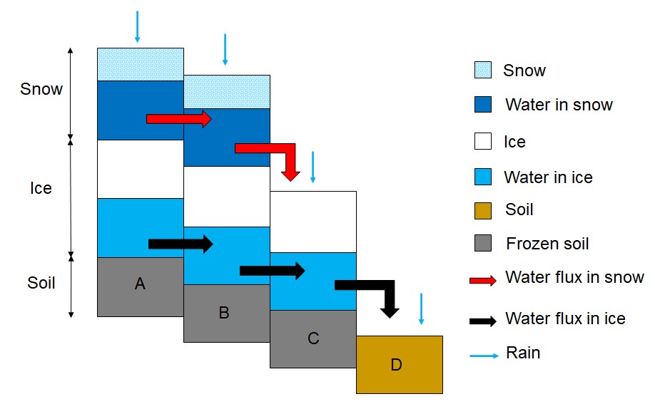
Fig. 5.1 Vertical and lateral fluxes interconnection scheme on cells covered by snow and ice (A,B), only covered by ice (C), and free from snow and ice (D).

BOX 5.A Glaciers initial conditions

Initial conditions require two information: the glaciers area and the ice (water equivalent) thickness in each cell.

For the first request, the GLIMS project (www.glims.org) allows to obtain the most recent mapping of glaciers around the world.

The best way to have information about glaciers thickness is to do direct measurements, as radio-echo soundings, but this kind of measures are very difficult and unusual over large areas. In literature several approaches to estimate glaciers thickness have been developed. One method use volume-area scale relations for glaciers (Chen and Ohmura, 1990), this allows to obtain the mean ice thickness over the entire glacier. Other methods involve principles of ice flow mechanics and require knowledge of surface velocity field, as the one developed by Farinotti et al., 2009; despite the accuracy of this method, such a physical modelling approach requires an onerous input data set and can only be applied to well-monitored glacier system.

Another class of methods employs the perfect plasticity assumption coming from Nye’s (1952) theory for the flow mechanics of an infinitely wide glacier (Aleynikov et al., 2002; Wallinga and van de Wal, 1998; Hoelzle et al., 2003; Li et al., 2012). The Nye’s theory revised by Aleynikov et al. (2002) is simple, it doesn’t involve onerous calculation and data request, but allows to maintain the raster based approach, characterizing each iced cell with the correspondent ice thickness. The ice thickness is calculated with equation (5.3), knowing the local slope \(\alpha\) , the average density of ice, \(\rho\) (equal to 840 kg/m3), the gravity acceleration , \(g\), and the maximum possible shear stress, \(\tau_{P}\) (equal to 0.10 MPa).

(5.3)\[h = \ \frac{\tau_{P}}{\rho\ g\ \sin\alpha}\]

However, this formulation is valid only for plane areas with \(l\ > \ 5h\); for the remaining areas, where approximation of a glacier by a plane-parallel plate is inappropriate, the maximum thickness of the glacier would be higher in comparison with calculation made with equation (5.3). The corrected thickness, \(h_{c}\), is obtained by inserting a coefficient depending on the glacier width, \(b\):

(5.4)\[h_{c} = \ \frac{1 + h}{b}\frac{\tau_{P}}{\rho\ g\ \sin\alpha}\]

where \(h\) represents the results of the calculation according to equation (5.3).