9. Discharge routing

9.1. Channel routing

Discharge routing is computed according to the variable parameter Muskingum-Cunge-Todini method (MCT; Todini, 2007), applied to every cell of the computation domain with length \(\mathrm{\Delta}x\).

The outflow \(O_{t + \mathrm{\Delta}t}\) from a reach segment of length \(\mathrm{\Delta}x\) is given by a linear combination of variable coefficients and the inflow, \(I\), and outflow at time \(t\) and \(t + \mathrm{\Delta}t\).

(9.1)\[O_{t + \mathrm{\Delta}t} = C_{1}\ I_{t + \mathrm{\Delta}t} + \ C_{2}\ I_{t} + \ C_{3}\ O_{t}\ {+ \ C}_{4}\ Q_{l}\]

where \(Q_{l}\) is lateral inflow. The coefficients expressed in terms of corrected Courant \(C^{*}\) and Reynolds \(D^{*}\) numbers are given by the following expressions:

(9.2)\[C_{1} = \ \frac{- 1 + C_{t + \mathrm{\Delta}t}^{*} + \ D_{t + \mathrm{\Delta}t}^{*}}{1 + C_{t + \mathrm{\Delta}t}^{*} + \ D_{t + \mathrm{\Delta}t}^{*}}\]

(9.3)\[C_{2} = \ \frac{1 + C_{t}^{*} - \ D_{t}^{*}}{1 + C_{t + \mathrm{\Delta}t}^{*} + \ D_{t + \mathrm{\Delta}t}^{*}}\ \bullet \ \frac{C_{t + \mathrm{\Delta}t}^{*}}{C_{t}^{*}}\]

(9.4)\[C_{3} = \ \frac{1 - C_{t}^{*} + \ D_{t}^{*}}{1 + C_{t + \mathrm{\Delta}t}^{*} + \ D_{t + \mathrm{\Delta}t}^{*}}\ \bullet \ \frac{C_{t + \mathrm{\Delta}t}^{*}}{C_{t}^{*}}\]

(9.5)\[C_{4} = \ \frac{2\ C_{t + \mathrm{\Delta}t}^{*}}{1 + C_{t + \mathrm{\Delta}t}^{*} + \ D_{t + \mathrm{\Delta}t}^{*}}\]

with

(9.6)\[C_{t}^{*} = \ \frac{c_{t}}{\beta_{t}}\ \bullet \frac{\mathrm{\Delta}t}{\mathrm{\Delta}x}\]

(9.7)\[C_{t + \mathrm{\Delta}t}^{*} = \ \frac{c_{t + \mathrm{\Delta}t}}{\beta_{t + \mathrm{\Delta}t}}\ \bullet \frac{\mathrm{\Delta}t}{\mathrm{\Delta}x}\]

(9.8)\[D_{t}^{*} = \ \frac{Q_{t}}{\beta_{t}\ B\ S_{0}\ c_{t}\ \mathrm{\Delta}x}\ \]

(9.9)\[D_{t + \mathrm{\Delta}t}^{*} = \ \frac{Q_{t + \mathrm{\Delta}t}}{\beta_{t + \mathrm{\Delta}t}\ B\ S_{0}\ c_{t + \mathrm{\Delta}t}\ \mathrm{\Delta}x}\]

where \(c\) is the wave celerity, \(B\) is channel topwidth, \(S_{0}\) is reach bed slope, and \(\beta = \ \frac{c\ \ A}{Q}\) a dimensionless correcting factor.

A first guess estimate \({\widehat{O}}_{t + \mathrm{\Delta}t}\) for the outflow \(O_{t + \mathrm{\Delta}t}\) at time \(t + \mathrm{\Delta}t\) is initially computed as:

(9.10)\[{\widehat{O}}_{t + \mathrm{\Delta}t} = \ O_{t} + \ \left( I_{t + \mathrm{\Delta}t} - \ I_{t} \right)\]

where \(O_{t}\) is outflow a time \(t\), \(I_{t + \mathrm{\Delta}t}\) and \(I_{t}\) are inflow at time \(t + \mathrm{\Delta}t\), and \(t\), respectively.

Then the reference discharge is computed at time \(t\), and \(t + \mathrm{\Delta}t\) as:

(9.11)\[Q_{t} = \frac{I_{t} + O_{t}}{2}\]

(9.12)\[Q_{t + \mathrm{\Delta}t} = \frac{I_{t + \mathrm{\Delta}t} + {\widehat{O}}_{t + \mathrm{\Delta}t}}{2}\]

and the reference water levels, \(y\) (normal depth), can be derived by means of a Newton-Raphson approach from the following implicit equations:

(9.13)\[y_{t} = y\left\{ Q_{t},\ n,\ S_{0} \right\}\]

(9.14)\[y_{t + \mathrm{\Delta}t} = y\left\{ Q_{t + \mathrm{\Delta}t},\ n,\ S_{0} \right\}\]

where \(n\) is Manning roughness coefficient, and \(\ S_{0}\) is bed slope. Details of the Newton-Raphson procedure can be found in Box 9.A.

BOX 9.A The Newton-Raphson algorithm to derive the normal depth

When the stage y is to be derived from a known discharge value \(Q^{*}\) in a channel, a non-linear implicit problem must be solved, except in the case of a very wide rectangular section for which the solution becomes trivial. Since a direct closed solution is not generally available, several numerical approaches to find the zeroes of a non-linear function can be used, such as the bisection or the Newton-Raphson methods. In this case, given that the involved functions are continuous and differentiable (triangular, rectangular and trapezoidal cross sections), a simple Newton-Raphson algorithm can be used. The problem reduces to finding the zeroes of the following function of \(y\) :

(9.15)\[f(y) = \ Q(y) - Q^{*} = 0\ \]

where \(Q(y)\) (L³ T⁻¹) is defined as:

(9.16)\[Q(y) = \ \frac{\sqrt{S_{0}}}{n}\ \frac{A\ (y)^{\frac{5}{3}}}{P\ (y)^{\frac{2}{3}}}\]

with \(S_{0}\) (dimensionless) the bottom slope, \(n\) the Manning friction coefficient (L^(1/3) T⁻¹), \(A(y)\) (L²) the wetted area, and \(P(y)\) (L) the wetted perimeter.

The Newton-Raphson algorithm, namely:

(9.17)\[y_{i + 1} = y_{i} - \ \frac{f\left( y_{i} \right)}{f^{'}\left( y_{i} \right)}\]

allows one to find the solution to the problem with a limited number of iterations starting from an initial guess \(y_{0}\) and can be implemented in this case by defining:

(9.18)\[f\left( y_{i} \right) = Q\left( y_{i} \right) - Q^{*} = \ \frac{\sqrt{S_{0}}}{n}\ \frac{A\ \left( y_{i} \right)^{\frac{5}{3}}}{P\ \left( y_{i} \right)^{\frac{2}{3}}}\ - Q^{*}\]

And taking the first derivative

(9.19)\[f^{'}(y) = \frac{d\left\lbrack Q(y) - Q^{*} \right\rbrack}{dy}|_{y = y_{i}} = \ \frac{dQ(y)\ }{dy}|_{y = y_{i}} = \ \frac{5}{3}\ \frac{\sqrt{S_{0}}}{n}\ \left\lbrack \frac{A(y)}{P(y)} \right\rbrack^{\frac{2}{3}}\ \left\lbrack B(y) - \frac{4}{5}\ \frac{A(y)}{P(y)\ \sin\alpha} \right\rbrack = B(y)\ c(y)\]

All quantities appearing in Equation 9-19 are provided in analytical form for geometric sections in Box 9.B.

Using the reference discharge and water level it is then possible to estimate all the other quantities at times \(t\) and \(t + \mathrm{\Delta}t\).

The celerity:

(9.20)\[c_{t} = c\ \left\{ Q_{t},\ y_{t},\ n,\ S_{0} \right\}\]

(9.21)\[c_{t + \mathrm{\Delta}t} = c\ \left\{ Q_{t + \mathrm{\Delta}t},\ y_{t + \mathrm{\Delta}t},\ n,\ S_{0} \right\}\]

the actual expressions for the celerity valid for triangular, rectangular and trapezoidal cross sections, are given in BOX 9.B.

The correcting factor, \(\beta\):

(9.22)\[\beta_{t} = \ \frac{c_{t}\ A_{t}}{Q_{t}}\]

(9.23)\[\beta_{t + \mathrm{\Delta}t} = \ \frac{c_{t + \mathrm{\Delta}t}\ A_{t + \mathrm{\Delta}t}}{Q_{t + \mathrm{\Delta}t}}\]

The corrected Courant numbers, and cell Reynolds numbers, from Equations (9.6) ÷ (9.9), and the weight coefficients, \(C_{1}\) ÷ \(C_{4}\), from (9.2) ÷ (9.5). The outflow is finally computed with Equation (9.1).

It is advisable to repeat twice the computation of outflow starting from Equation (9.11), in order to eliminate the influence of the first guess \({\widehat{O}}_{t + \mathrm{\Delta}t}\) given by Equation (9.10).

Storage, \(S\), at time \(t + \mathrm{\Delta}t\) can be estimated as:

(9.24)\[S_{t + \mathrm{\Delta}t} = \ \frac{\left( 1 - D_{t + \mathrm{\Delta}t}^{*} \right)\ \mathrm{\Delta}t}{2\ \ C_{t + \mathrm{\Delta}t}^{*}}\ I_{t + \mathrm{\Delta}t} + \ \frac{\left( 1 + D_{t + \mathrm{\Delta}t}^{*} \right)\ \mathrm{\Delta}t}{2\ \ C_{t + \mathrm{\Delta}t}^{*}}\ O_{t + \mathrm{\Delta}t}\]

Eventually, the water stage can be estimated, by taking into account that the Muskingum model is a lumped model in space, which means that the water level will represent the “average” water level in the reach.

Firstly the average wetted area in the river reach is estimated as:

(9.25)\[{\overline{A}}_{t + \mathrm{\Delta}t} = \ \frac{S_{t + \mathrm{\Delta}t}}{\mathrm{\Delta}x}\ \]

from which, knowing the shape of the cross section, the water stage can be evaluated:

(9.26)\[\ y_{t + \mathrm{\Delta}t\ } = y\ \left\{ {\overline{A}}_{t + \mathrm{\Delta}t} \right\}\]

Equation (9.26) represents the average water stage in the reach and, on the basis of the Muskingum wedge assumption can be interpreted as the water stage more or less in the centre of the reach.

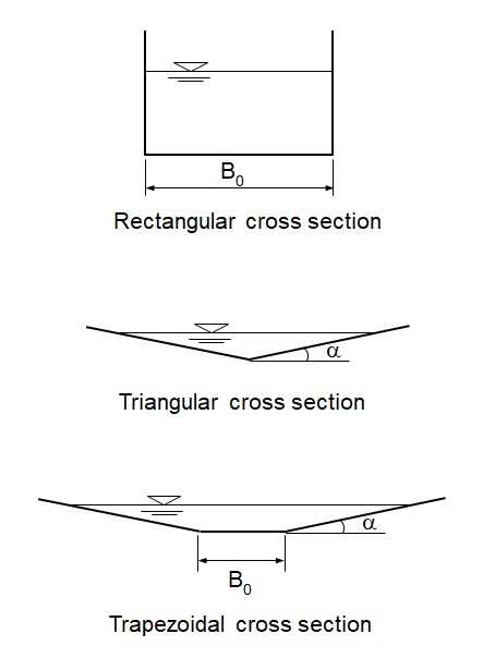
BOX 9.B Hydraulic properties for triangular, rectangular and trapezoidal cross sections

Given the cross-sections in the Figure below, the following equations can be used to represent a generic triangular, rectangular or trapezoidal cross section.

(9.27)\[A(y) = \ \left( B_{0} + y\ \cot\alpha \right)\ \ y\]

the wetted area (L²)

(9.28)\[B(y) = \ B_{0} + 2\ y\ \cot\alpha\ \]

the surface width (L)

(9.29)\[P(y) = \ B_{0} + \frac{2\ y}{\sin\alpha}\ \ \]

the wetted perimeter (L) with \(B_{0}\) the bottom width (L) (\(B_{0} = 0\) for the triangular cross section) and \(y\) the water stage (L).

The velocity (L T⁻¹) is computed as:

(9.30)\[v(y) = \ \frac{Q(y)}{A(y)} = \ \ \ \frac{\sqrt{S_{0}}}{n}\ \frac{A\ (y)^{\frac{2}{3}}}{P\ (y)^{\frac{2}{3}}}\]

celerity (L T⁻¹) is calculated as:

(9.31)\[c(y) = \ \frac{dQ(y)}{dA(y)} = \ \ \frac{1}{B(y)}\ \frac{dQ(y)}{dy} = \frac{5}{3}\frac{\sqrt{S_{0}}}{n}\ \frac{A\ (y)^{\frac{2}{3}}}{P\ (y)^{\frac{2}{3}}}\ \left( 1 - \frac{4}{5}\ \frac{A(y)}{B(y)\ P(y)\ \sin\alpha} \right)\]

The correction factor is calculated as:

(9.32)\[\beta(y) = \ \frac{c(y)}{v(y)} = \frac{5}{3}\ \left( 1 - \frac{4}{5}\ \frac{A(y)}{B(y)\ P(y)\ \sin\alpha} \right)\]

The three cross sections shapes (rectangular, triangular and trapezoidal)

9.2. Level pool routing

Reservoirs and lakes can be modeled as a pool. Level pool routing is a procedure for calculating the outflow hydrograph from a reservoir with a horizontal water surface, given its inflow hydrograph and storage-outflow characteristics (Fiorentini and Orlandini, 2013).

The equations governing reservoir dynamics can be combined to yield the nonlinear first-order ordinary differential equation

(9.33)\[\frac{dS}{dt} = I(t) - Q(t,S)\]

where \(\text{S}\) is the volume of water stored in the reservoir, \(t\) is the time, \(I\) is the inflow discharge, and \(Q\) is the outflow discharge, or the equivalent differential equation

(9.34)\[\frac{dH}{dt} = \frac{I(t) - Q(t,H)}{A(H)}\]

where \(H\) is the water surface level and \(A = \ \frac{dS}{dh}\) is the water surface area at elevation \(H\).

The storage function \(S = S(h)\) relating water surface level \(H\) and reservoir storage \(S\) can be determined by using topographic maps or by processing digital elevation models. The outflow function \(Q = Q(t,H)\) can be derived from hydraulic equations relating the head \(H\) to the outflow discharge \(Q\). Physical modeling may be necessary in all those cases in which the (gated) bottom outlets (sluice gates) and/or spillways involved cannot be (entirely) characterized in a conceptual manner.

Equation (9.33) can be solved analytically under the assumptions that the storage-outflow discharge relationship can be expressed in the form of a power function and input discharge is represented by simple functions. In most of the cases of practical relevance, however, Equation (9.33) and Equation (9.34) need to be solved numerically. Runge-Kutta method is numerical method often employed for this purpose (Carnahan et al., 1969; Chow et al., 1988).

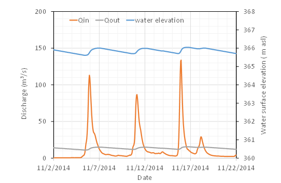
BOX 9.C Idro lake simulation

Lake Idro, or Eridio, is a lake of glacial origin located in the province of Brescia on the border with Trentino, in Northern Italy. Situated at 368 meter above sea level, it is formed by the waters of the Chiese river which is also its outlet. Its surface is 10.9 km² and reaches a maximum depth of 122 meter.

Lake Idro is the first natural Italian lake, to have been subjected to artificial regulation. The original idea of constructing a dam dates back to 1855, but the concession was given jointly to Società Elettrica Bresciana (SEB) and the University of Naviglio Grande Bresciano in 1917 to reduce Lake Idro to a regulated reservoir, in order to produce electricity and have greater volumes of water for the summer irrigation of the Brescia and Mantua areas. The regulation work was built in the 1920s and came into operation in 1933.

Input and output discharge and water elevation of the Idro lake simulated by the FeST model

9.2.1. Third order Runge-Kutta method

To solve Equation (9.34) using a third-order integration scheme, three small increments of the independent variable, time, using known values of the dependent variable \(H\) are made. The water elevation \(H\) at the (j + 1)^(th) time step is expressed as

(9.35)\[H_{j + 1} = H_{j} + \frac{1}{4}\left( \Delta H_{1} + 3\Delta H_{3} \right)\]

where the three successive approximations are estimated as

(9.36)\[\Delta H_{1} = \frac{I\left( t_{j} \right) - Q\left( H_{j} \right)}{A_{r}\left( H_{j} \right)}\Delta t\]

(9.37)\[\Delta H_{2} = \frac{I\left( t_{j} + \frac{\Delta t}{3} \right) - Q\left( H_{j} + \frac{\Delta H}{3} \right)}{A_{r}\left( H_{j} + \frac{\Delta H}{3} \right)}\Delta t\]

(9.38)\[\Delta H_{3} = \frac{I\left( t_{j} + 2\frac{\Delta t}{3} \right) - Q\left( H_{j} + 2\frac{\Delta H}{3} \right)}{A_{r}\left( H_{j} + 2\frac{\Delta H}{3} \right)}\Delta t\]

9.2.2. Fourth order Runge-Kutta method

To solve Equation (9.34) using a fourth-order integration scheme, four small increments of the independent variable, time, using known values of the dependent variable \(H\) are made. The water elevation \(H\) at the (j + 1)^(th) time step is expressed as

(9.39)\[H_{j + 1} = H_{j} + \frac{1}{6}\left( \mathrm{\Delta}H_{1} + 2 \bullet \mathrm{\Delta}H_{2} + 2 \bullet \mathrm{\Delta}H_{3} + \mathrm{\Delta}H_{4} \right)\]

where the four successive approximations are estimated as

(9.40)\[\mathrm{\Delta}H_{1} = \frac{I\left( t_{j} \right) - Q(H_{j})}{A_{r}\left( H_{j} \right)} \bullet \mathrm{\Delta}t\]

(9.41)\[\mathrm{\Delta}H_{2} = \frac{I\left( t_{j} + \frac{1}{2}\mathrm{\Delta}t \right) - Q(H_{j} + \frac{1}{2}\mathrm{\Delta}H_{1})}{A_{r}\left( H_{j} + \frac{1}{2}\mathrm{\Delta}H_{1} \right)} \bullet \mathrm{\Delta}t\]

(9.42)\[\mathrm{\Delta}H_{3} = \frac{I\left( t_{j} + \frac{1}{2}\mathrm{\Delta}t \right) - Q(H_{j} + \frac{1}{2}\mathrm{\Delta}H_{2})}{A_{r}\left( H_{j} + \frac{1}{2}\mathrm{\Delta}H_{2} \right)} \bullet \mathrm{\Delta}t\]

(9.43)\[\mathrm{\Delta}H_{4} = \frac{I\left( t_{j} + \mathrm{\Delta}t \right) - Q(H_{j} + \mathrm{\Delta}H_{3})}{A_{r}\left( H_{j} + \mathrm{\Delta}H_{3} \right)} \bullet \mathrm{\Delta}t\]