6. Infiltration and runoff

Infiltration is the process by which water on the ground surface enters the soil. It is commonly used in both hydrology and soil sciences (Haghaibi et al., 2011).

Infiltration is caused by multiple factors including; gravity, capillary forces, adsorption, and osmosis. Many soil characteristics can also play a role in determining the rate at which infiltration occurs.

Infiltration takes place in the vadose zone, also termed the unsaturated zone. It is the part of Earth between the land surface and the top of the phreatic zone, the position at which the groundwater (the water in the soil’s pores) is at atmospheric pressure (“vadose” is from the Latin word for “shallow”). Hence, the vadose zone extends from the top of the ground surface to the water table.

Water in the vadose zone has a pressure head less than atmospheric pressure and is retained by capillary action. If the vadose zone envelops soil, the water contained therein is termed soil moisture. In fine grained soils, capillary action can cause the pores of the soil to be fully saturated above the water table at a pressure less than atmospheric. The vadose zone does not include the area that is still saturated above the water table, often referred to as the capillary fringe.

The description of water flow in the vadose zone is quite complicated as compared to the saturated zone (Merdun, 2012). An accurate description of soil hydraulic properties is the main limitation for a good description of water processes under unsaturated flow conditions in particular when implemented for large study areas. This led many researchers to simplify the description of water movement as one dimensional vertical process though it is a three dimensional.

Several infiltration models exist in the literature that exhibit different levels of accuracy. These models are usually based on Richards equation (Richards, 1931; Lassabatere et al., 2009). Richards equation provides an appropriate tool to describe the infiltration process with a detailed description of the flow and water distribution within the soil profile (Tinet et al., 2015). Numerical solutions based on finite difference, finite element or boundary element techniqueshave been used to solve Richards equation (Feddes et al., 1988). Due to the non-linearity of the described process as well as the high detail of soil hydraulic parameters requirements, the use of numerical solutions is considered as time consuming and facing some stability problems (Tinet et al., 2015). Despite the progress made for developing efficient numerical schemes joined with faster computers, the use of such numerical methods is still time consuming when implemented for large study areas (Ross, 2003).

Several simplifications have been suggested to model the infiltration process. These models are commonly categorized into empirical, semi-empirical and physically based (Mishra et al., 2003). Empirical models are formulated as simple equation, derived from actual field measured infiltration data through curve fitting (Ravi and Williams, 1998). Examples of these models are: SCS-CN (SCS, 1985), Kostiatov (1932), Collis-George (1977), Huggins and Monke (1966), etc. Many existing hydrological models in the literature are based on these empirical models, in particular the SCS-CN such as: ANSWERS (Beasely and Huggins, 1980), EPIC (Sharplay and Williams, 1990), SWAT (Arnold et al., 2012), Etc. Many semi-empirical or approximations models exist for example: Green and Ampt (1911), Philip (1957), Smith and Parlange (1978), etc. These models allow a simplification of this process through some assumptions made either for soil hydraulic properties or for the boundary conditions (Lassabatère et al., 2009).

BOX 6.A The ponding time

According to Brutsaert (2005), ponding time is a term used in hydrology for a saturated soil surface (from rain) and occurs water puddle. When it rains, the water will be puddling if the intensity of the rain exceeds the value of the infiltration capacity of the soil that receives rain. Ponding time (\(t_{p}\)) is the time from the beginning of rainwater infiltration until surface runoff occurs, starting from the beginning of the rain occurs until the water begins to puddle on the soil surface. Time before ponding occurs (\(t < t_{p}\)), the intensity of rain is less than the potential rate of soil infiltration and the soil surface in unsaturated conditions. Ponding begins to occur when the intensity of rain exceeds the infiltration rate. At this time(\(t = t_{p}\)), the soil surface begins to saturate with water. As the rain continues(\(t > t_{p}\)), the soil saturated zone will deepen and the surface runoff begins to occur from the puddle.

BOX 6.B The Brooks and Corey water retention curve

Water retention curve is the relationship between the water content, \(\theta\), and the soil water potential (suction), \(\psi\). This curve is characteristic for different types of soil, and is also called the soil moisture characteristic. At potentials close to zero, a soil is close to saturation, and water is held in the soil primarily by capillary forces. As \(\theta\) decreases, binding of the water becomes stronger, and at small potentials (more negative, approaching wilting point) water is strongly bound in the smallest of pores, at contact points between grains and as films bound by adsorptive forces around particles.

The shape of water retention curves can be characterized by several models, one of them known as the Brooks and Corey (1964):

(6.1)\[\frac{\theta - \theta_{r}}{\theta_{s} - \theta_{r}}\mathbf{=}\ \left( \frac{\psi}{\psi_{a}} \right)^{B}\]

where \(\theta_{r}\) and \(\theta_{s}\) represent the residual and saturated soil moisture, respectively, (m³/m³),

\(\psi\) represents the soil suction (m), \(\psi_{a}\) represents the air-entry pressure (m), and \(B\) is the pore size distribution index (-).

Equation for hydraulic conductivity of partially saturated soil, \(K(\psi)\) (m/s), is:

(6.2)\[\begin{split}K(\psi) = \left\{ \begin{aligned} & K_{s}\left( \frac{\psi_{a}}{\psi} \right)^{2 + 3B}\psi \leq \psi_{a} \\ & K_{s}\ \ \ \ \ \ \ \ \ \ \ \ \ \ \ \ \ \ \ \psi > \psi_{a} \\ \end{aligned} \right.\ \end{split}\]

where \(K_{s}\) (m/s) is hydraulic conductivity of saturated soil.

6.1. The SCS Curve Number

The SCS Curve Number (SCS-CN) (SCS, 1985) is one of widely implemented models for the calculation of surface runoff. According to this method, the infiltration is calculated as the difference between the precipitation and the runoff. SCS-CN method does not consider the rainfall intensity or duration; it only considers the total precipitation.

(6.3)\[I = P_{tot} - R \]

(6.4)\[R = \frac{{(P - I_{a})}^{2}}{P - I_{a} + S}\]

with

(6.5)\[I_{a} = 0.2\ S\]

where \(\mathbf{I}\) is the total infiltration [L], \(P\) is the precipitation [L], \(R\) is the runoff [L], \(S\) is the maximum retention capacity [L], and \(I_{a}\) is the initial abstraction. \(S\) and \(CN\) are related.

(6.6)\[S = \ S_{0}\left( \frac{100}{CN} - 1 \right)\]

with \(S_{0} = 254\) mm. The fraction of precipitation that is not converted to runoff is accounted for as infiltration

The \(CN\) parameter values were derived from the curves of the plotted relationship between the rainfall and the runoff. The \(CN\) is mainly related to the land use. The \(CN\) value is adjusted according to the antecedent moisture conditions. \({CN}_{II}\) stands for average soil moisture conditions (AMC II) of the previous 5 days, \({CN}_{I}\) stands for dry soil moisture conditions AMC I and \({CN}_{III}\) stands for wet soil moisture conditions AMC III. The SCS-CN approach has been subjected to several modifications in order to be adopted for various land uses and climatic conditions (Soulis and Valiantzas, 2012). Many researchers have proposed a modified version of the SCS-CN for continuous simulations (Adornado and Yoshida, 2010). The method proposed by Ravazzani et al. (2007) has been implemented within the FeST model. According to this method at each time step, \(S\) is calculated depending on the soil degree of saturation, \(\varepsilon_{t}\)

(6.7)\[S = S_{1} - \varepsilon(S_{1} - S_{3})\]

with

(6.8)\[S_{1} = S({CN}_{I})\]

(6.9)\[{S\ }_{3} = S({CN}_{III})\]

(6.10)\[{CN}_{I} = \ {CN}_{II} - \ \left( 20\ \frac{100\ - \ {CN}_{II}}{100 - \ {CN}_{II} + EXP\left( 2.533 - 0.0636\ \left( 100 - \ {CN}_{II} \right) \right)} \right)\]

(6.11)\[{CN}_{III} = {CN}_{II}\ EXP\ \left( 0.00673\ \left( 100 - \ {CN}_{II} \right) \right)\]

(6.12)\[\varepsilon_{t} = \frac{\theta_{t} - \theta_{r}}{\theta_{s} - \theta_{r}}\]

where \(\theta_{t}\) is the actual water content at time \(t\) [L³/L³], \(\theta_{s}\) is the saturated water content [L³/L³] and \(\theta_{r}\) is the residual water content [L³/L³].

\(S\) in equation (6.7) is updated in each cell at the beginning of a storm event, and it is kept constant till the end of the storm. The \({CN}_{II}\) parameters values, function of CORINE land cover class (https://land.copernicus.eu/user-corner/technical-library/clc-product-user-manual), and hydrological class is reported in Table 6.1.

Table 6.1 The \({CN}_{II}\) parameter values as a function of CORINE land cover class and hydrological class (A, B, C, and D)

CORINE code	Description	A	B	C	D
111	Continuous urban fabric	77	85	90	92
112	Discontinuous urban fabric	57	72	81	86
121	Industrial or commercial units	89	90	94	94
122	Road and rail networks and associated land	98	98	98	98
123	Port areas	89	92	94	94
124	Airports	81	88	91	93
131	Mineral extraction sites	46	69	79	84
132	Dump sites	46	69	79	84
133	Construction sites	46	69	79	84
141	Green urban areas	39	61	74	80
142	Sport and leisure facilities	39	61	74	80
211	Non-irrigated arable land	70	80	86	90
212	Permanently irrigated land	85	90	92	94
213	Rice fields	100	100	100	100
221	Vineyards	45	66	77	83
222	Fruit trees and berry plantations	45	66	77	83
223	Olive groves	45	66	77	83
231	Pastures	30	58	71	78
241	Annual crops associated with permanent crops	58	73	82	87
242	Complex cultivation patterns	58	73	82	87
243	Land principally occupied by agriculture, with significant areas of natural vegetation	52	70	80	84
244	Agro-forestry areas	58	73	82	87
311	Broad-leaved forest	36	60	73	79
312	Coniferous forest	36	60	73	79
313	Mixed forest	36	60	73	79
321	Natural grassland	49	69	79	84
322	Moors and heathland	49	69	79	84
323	Sclerophyllous vegetation	49	69	79	84
324	Transitional woodland/shrub	36	60	73	79
331	Beaches, dunes, sands	76	85	89	91
332	Bare rock	77	86	91	94
333	Sparsely vegetated areas	49	69	79	84
334	Burnt areas	77	86	91	94
335	Glaciers and perpetual snow	100	100	100	100
411	Inland marshes	100	100	100	100
412	Peatbogs	100	100	100	100
421	Salt marshes	100	100	100	100
422	Salines	100	100	100	100
423	Intertidal flats	100	100	100	100
511	Water courses	100	100	100	100
512	Water bodies	100	100	100	100
521	Coastal lagoons	100	100	100	100
522	Estuaries	100	100	100	100
523	Sea and ocean	100	100	100	100

6.2. Philip

Philip proposed a semi analytical solution (Philip, 1957) to solve the non-linear partial differential Richards equation (Richards, 1931). The infiltration capacity, \(i^{*}\), as expressed by Philip’s equation is approximated by

(6.13)\[i^{*}(t) = \frac{1}{2}S_{i} \cdot t^{- \frac{1}{2}} + C_{S,3} \cdot K_{s}\]

where \(S_{i}\) is a parameter called sorptivity (m/s²), which is a function of the soil suction potential, \(t\) is the time from the beginning of infiltration process (s), \(K_{s}\) is the hydraulic conductivity (m/s), and \(C_{S,3}\) is a constant. The sorptivity is considered as capacity of the soil to uptake or release water.

An analytic expression of \(S_{i}\) and \(C_{S,3}\) is given by Sivapalan et al. (1987):

(6.14)\[C_{S,3} = \frac{1}{2}\ \left( 1 + \theta_{rs,i}^{\eta} \right)\]

where

(6.15)\[\eta = \frac{2 + 3 \cdot B}{B}\]

(6.16)\[\theta_{rs,i} = \frac{\theta_{i} - \theta_{r}}{\theta_{s} - \theta_{r}}\]

where \(B\) is the Brooks and Corey (1964) pore size distribution index, \(\theta_{i}\) is the soil water content at the beginning of the infiltration, \(\theta_{s}\) and \(\theta_{r}\) are the water content at saturation and residual, respectively.

(6.17)\[S_{i} = \left\lbrack \frac{2 \cdot K_{s}\left( \theta_{s} - \theta_{i} \right)^{2}\psi_{c}}{\left( \theta_{s} - \theta_{r} \right)}\left( \frac{1}{\eta + \frac{1}{2}B - 1} + \frac{\theta_{s} - \theta_{r}}{\theta_{s} - \theta_{i}} \right) \right\rbrack^{\frac{1}{2}}\]

where \(\psi_{c}\) is the soil suction head (bubbling pressure) (m).

According to Milly (1986), under the assumption of time compression approximation, infiltration capacity can be expressed as a function of cumulative infiltration:

(6.18)\[i^{*}(i_{c}) = C_{S,3} \cdot K_{s}\left( 1 + \left\lbrack \left( 1 + \frac{4 \cdot C_{S,3} \cdot K_{s} \cdot i_{c}}{S_{i}^{2}} \right)^{\frac{1}{2}} - 1 \right\rbrack^{- 1} \right)\]

where \(i_{c}\) is the cumulative infiltration computed by integrating the infiltration amount from the beginning of the precipitation event.

The actual infiltration rate, \(i\), is computed as the minimum between infiltration capacity and rainfall rate, \(Rain\) :

(6.19)\[i = \min\left\lbrack i^{*}(i_{c}),Rain \right\rbrack\]

When rain rate exceeds infiltration capacity, the rainfall excess is transformed to runoff.

BOX 6.C The time compression approximation

Infiltration capacity is the maximum infiltration rate that results when rainfall intensity is so large that the surface is saturated (i.e., ponded) instantaneously. Actual infiltration rate is typically lower due to the limited water supply to the soil surface, especially during early times during typical rainfall events. Indeed, infiltration capacity starts out large during early times, and as more and more rainfall infiltrates, infiltration capacity decreases with time. The decreasing infiltration capacity eventually becomes equal to the rainfall intensity, and surface runoff (and ponding) is initiated. Ponding time is defined as the time after the beginning of rainfall at which ponding or surface runoff occurs (Diskin and Nazimov, 1996). From that time onward, with continued rainfall, the surface remains ponded, and so actual infiltration rate remains equal to infiltration capacity but continues to decrease with time until (in the long term) it reaches a constant rate asymptotically, provided the soil is sufficiently deep. The infiltration theory suggests the early-time infiltration behavior is governed by absorption (due to capillary action of soil), while late-time behavior is governed by gravitational action, and that the final constant infiltration rate after a long time is approximately equal to the saturated hydraulic conductivity of the soil (Brutsaert, 2005).

However, rainfall intensity is seldom larger than infiltration capacity at early times (Assouline, 2013), and therefore, initially, all rainfall infiltrates. To account for this discrepancy, the time compression approximation (TCA), also referred to as time condensation approximation, was introduced to estimate both ponding time and the postponding infiltration rate. The essential concept behind TCA is the assumption of a unique, invariant relationship between infiltration capacity and the cumulative infiltration volume, regardless of the rainfall (or infiltration) history. The infiltration rate and cumulative infiltration volume after ponding could be obtained by shifting the time of infiltration capacity and cumulative potential infiltration over a compression reference time, respectively (Brutsaert, 2005); this explains the name “time condensation approximation”.

6.3. Green and Ampt

Green and Ampt (1911) derived an approximate mechanistic model for infiltration under ponded condition into a deep homogeneous soil with uniform initial moisture content which assumes a piston-type water content profile with a well-defined wetting front. This model is based on the hypothesis that there is the existence of sharp wetting front having a constant matric potential and the wetting zone is uniformly wetted with a constant hydraulic conductivity (Fig. 6.1). The model can be derived by combining the Darcy’s law with the continuity principle. The resulting Green-Ampt equations is given as

(6.20)\[f(t) = K\ \left( 1 + \frac{h_{0} + h_{s}}{L} \right)\]

(6.21)\[F(t)\ - \ \left( h_{0} - h_{s} \right)\ \mathrm{\Delta}\theta\ ln\left( 1 + \frac{F(t)}{\left( h_{0} - h_{s} \right)\ \mathrm{\Delta}\theta\ }\ \right) = K\ t\]

where \(f(t) = \ \frac{dF(t)}{dt\ }\) is the infiltration rate; \(K\) is the effective hydraulic conductivity; \(h_{0}\) is the depth of ponding water over the soil surface; \(h_{s}\) is the capillary suction head at the wetting front; \(L\) is the depth of wetting front below the bottom of pond; \(F(t)\) is the cumulative infiltration depth; and \(\mathrm{\Delta}\theta = \ \phi_{e} - \ \theta_{i}\) is the soil moisture deficit; \(\phi_{e}\) is the effective porosity; and \(\theta_{i}\) is initial (antecedent) moisture content.

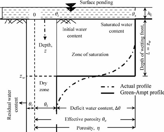
Fig. 6.1 Infiltration profile for the Green-Ampt model. Adapted from Kale and Sahoo, 2011.

Equation (6.20) is applicable only when water starts ponding on the soil surface from the beginning of the rainfall event. Therefore, to use this equation considering the condition of ponding some time after the start of rainfall, Mein and Larson (1973) developed a two-stage model for infiltration (under a constant-intensity rainfall) into a homogeneous soil with uniform initial moisture content. The first stage predicted the volume of infiltration at the moment when surface ponding begins. The second stage, which is used for prediction of infiltration after the occurrence of the ponding, described the subsequent infiltration behavior, wherein they provided the equations for the calculation of ponding time and accumulated infiltration depth. This variant of the Green-Ampt model of Mein and Larson (1973) can also be found in the referred textbooks (Chow et al. 1988).

The basic principles of the method are: in the absence of ponding, cumulative infiltration is calculated from cumulative rainfall; the potential infiltration rate at a given time is calculated from the cumulative infiltration at that time; and ponding has occurred when the potential infiltration rate is less than or equal to the rainfall intensity.

Consider a time interval from \(t\) to \(\mathrm{\Delta}t\). The rainfall intensity during this interval is denoted \(i_{t}\) and is constant throughout the interval. The potential infiltration rate and cumulative infiltration at the beginning of the interval are \(f(t)\) and \(F(t)\), respectively, and the corresponding values at the end of the interval are \(f(t + \ \mathrm{\Delta}t)\), and \(F(t + \ \mathrm{\Delta}t)\). It is assumed that \(f(t + \ \mathrm{\Delta}t)\) is known from given initial conditions or previous computation.

A flow chart for determining ponding time is presented in (Fig. 6.2).. There are three cases to be considered: (1) ponding occurs throughout the interval; (2) there is no ponding throughout the interval; and (3) ponding begins part-way through the interval. The infiltration rate is always either decreasing or constant with time, so once ponding is established under a given rainfall intensity, it will continue. Hence, ponding cannot cease in the middle of an interval, but only at its end point, when the value of the rainfall intensity changes.

The first step is to calculate the current potential infiltration rate \(f(t)\), from the known value of cumulative infiltration \(F(t)\):

(6.22)\[f(t) = K\ \left( \frac{h_{s\ }\mathrm{\Delta}\theta}{F(t)} + 1 \right)\]

The result \(f(t)\) is compared to the rainfall intensity \(i_{t}\). If \(f(t)\ \) is less than or equal to \(i_{t}\), case (1) arises and there is ponding throughout the interval. In this case the cumulative infiltration at the end of the interval, \(F(t + \ \mathrm{\Delta}t)\) is calculated from

(6.23)\[F(t + \ \mathrm{\Delta}t)\ - \ F(t) - \ h_{s\ }\mathrm{\Delta}\theta\ln\left( \frac{{F(t + \ \mathrm{\Delta}t) + \ h}_{s\ }\mathrm{\Delta}\theta}{F(t) + \ h_{s\ }\mathrm{\Delta}\theta} + 1 \right) = K\ \mathrm{\Delta}t\ \]

Both cases (2) and (3) have \(f(t)\ > \ \ i_{t}\) and no ponding at the beginning of the interval. Assume that this remains so throughout the interval; then, the infiltration rate is \(i_{t}\) and a tentative value for cumulative infiltration at the end of the time interval is

(6.24)\[F^{'}(t + \ \mathrm{\Delta}t)\ = \ F(t) + i_{t}\ \ \mathrm{\Delta}t\]

Next, a corresponding infiltration rate\(\ f^{'}(t + \ \mathrm{\Delta}t)\) is calculated from \(F^{'}(t + \ \mathrm{\Delta}t)\). If \(\ f^{'}(t + \ \mathrm{\Delta}t)\) is greater than \(i_{t}\) , case (2) occurs and there is no ponding throughout the interval.

Thus \(F(t + \ \mathrm{\Delta}t) = \ F^{'}(t + \ \mathrm{\Delta}t)\) and the problem is solved for this interval.

If \(\ f^{'}(t + \ \mathrm{\Delta}t)\) is is less than or equal to \(i_{t}\), ponding occurs during the interval (case (3)). The cumulative infiltration \(F(p)\) at ponding time is found by setting \(f(t) = \ \ i_{t}\) and \(F(t) = \ F(p)\) in equation (6.20) and solving for \(F(p)\) to give

(6.25)\[F(p)\ = \ \frac{K\ h_{s\ }\mathrm{\Delta}\theta\ }{i_{t} - K}\ \]

The ponding time is then \(t\ + \ \mathrm{\Delta}t^{'}\), where

(6.26)\[\mathrm{\Delta}t^{'} = \ \frac{F(p) - \ (t)}{i_{t}}\]

and the cumulative infiltration \(F(t + \ \mathrm{\Delta}t)\) is found by substituting \(F(t) = \ F(p)\) and \(\ \mathrm{\Delta}t = \ \mathrm{\Delta}t - \ \mathrm{\Delta}t^{'}\) in equation (6.23). The excess rainfall values are calculated by subtracting cumulative infiltration from cumulative rainfall, then taking successive differences of the resulting values. When rain rate exceeds infiltration capacity, the rainfall excess is transformed to runoff.

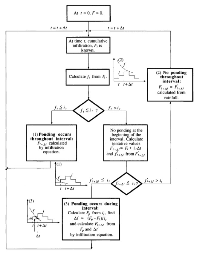
Fig. 6.2 Flow chart for determining infiltration and ponding time under variable rainfall intensity. (Chow et al., 1988)

BOX 6.D Soil hydrological parameter estimates based on soil texture

The following table reports soil hydrological parameter estimates (from Gowdish and Muñoz-Carpena, 2009; Rawls and Brakensiek, 1982, and Rawls et al., 1982).

USDA texture	\(\mathbf{K}_{\mathbf{s}}\)	\(\mathbf{\theta}_{\mathbf{s}}\)	\(\mathbf{\theta}_{\mathbf{r}}\)	\(\mathbf{B}\)	\(\mathbf{\theta}_{\mathbf{wp}}\)	\(\mathbf{\theta}_{\mathbf{fc}}\)	\(\mathbf{h}_{\mathbf{s}}\)	\(\mathbf{\psi}_{\mathbf{c}}\)
Clay	1.66E-07	0.475	0.090	0.165	0.272	0.296	0.623	0.373
Silty Clay	2.50E-07	0.479	0.056	0.150	0.250	0.317	0.578	0.342
Silty Clay-Loam	4.16E-07	0.432	0.040	0.177	0.208	0.300	0.538	0.326
Sandy Clay	3.33E-07	0.430	0.109	0.223	0.239	0.232	0.467	0.292
Sandy Clay-Loam	1.19E-06	0.330	0.068	0.177	0.148	0.187	0.424	0.281
Clay-Loam	6.38E-07	0.390	0.075	0.242	0.197	0.245	0.409	0.259
Silt	1.55E-06	0.450	0.020	0.200	0.140	0.240	0.350	0.210
Silt-Loam	1.88E-06	0.486	0.015	0.234	0.133	0.261	0.330	0.208
Loam	6.60E-07	0.434	0.027	0.252	0.117	0.200	0.175	0.112
Sand	5.83E-05	0.417	0.020	0.694	0.033	0.048	0.096	0.073
Loamy Sand	1.69E-05	0.401	0.035	0.553	0.055	0.084	0.120	0.087
Sandy Loam	7.19E-06	0.412	0.041	0.378	0.095	0.155	0.215	0.147

\(K_{s}\) hydraulic conductivity (m/s)

\(\theta_{s}\) saturated volumetric water content (m³/m³)

\(\theta_{r}\) residual volumetric water content (m³/m³)

\(B\) pore size distribution index

\(\theta_{wp}\) volumetric water contenta at the wilting point (m³/m³)

\(\theta_{wp}\) volumetric water contenta at the field capacity (m³/m³)

\(h_{s}\) suction at the wetting front (m)

\(\psi_{c}\) bubbling pressure (m)