11. Groundwater

The FeST model can simulate groundwater flow with a quasi 3D scheme based on macroscopic Cellular Automata (CA) (Ravazzani et al., 2011). CA represents a simple, attractive and alternative modelling technique respect to traditional numerical models that solve differential equations to describe complex phenomena (Toffoli, 1984). Cellular Automata are dynamical systems which are discrete in space and time, operate on a uniform, regular lattice and are characterised by local interactions. They were introduced by von Neumann (1966) to study self-reproducing systems and have been later used for modelling disparate complex physical phenomena (Di Gregorio, et al., 1999; Jimenez-Hornero et al., 2003; Parsons and Fonstad, 2007; Marshall and Randhir, 2008).

Many complex macroscopic fluid dynamical phenomena seem difficult to be modelled in these CA frames, because they take place on a large space scale and require a macroscopic level of description. Empirical CA methods were developed on the macroscopic scale in order to overcome this problem, dealing directly with the macroscopic variables (Di Gregorio and Serra, 1999; D’Ambrosio et al., 2001). These CA make use of local laws that are ruled by empirical parameters. As these latter can have no direct link with classical physical parameters, an accurate calibration phase is generally required (Iovine et al., 2005). At the contrary, physically based Macroscopic Cellular Automata (MCA), in which local rules derive directly by physical laws and depend on physical parameters, do not require a similar calibration (Bates and De Roo, 2000; Horritt and Bates, 2001; Mendicino et al., 2006).

11.1. Groundwater flow

Models based on CA paradigm consist of four primary components: a lattice of cells, the definition of a local neighbourhood area, transition rules determining the changes in cell properties, and boundary conditions (Parsons and Fonstad, 2007). To simulate water flux in unconfined aquifer, a two-dimensional lattice of cells is created. A value of saturated hydraulic conductivity, \(K_{s}\) [L T⁻¹], a value of specific yield, \(S_{y}\) [-], elevation of the bottom of the aquifer [L], and initial head [L] are assigned to each cell. The cell size must be small enough so that physical properties can be considered homogeneous in the cell space, but large enough to achieve macroscopic description of the physical processes. The cell size is set as \(\mathrm{\Delta}s = \ \mathrm{\Delta}x = \ \mathrm{\Delta}y\).

The neighbourhood in CA models defines the area of process influence. Among those proposed in literature for two-dimensional CA with square tessellation, as that here presented, the von Neumann and Moore ones are the most adopted: the von Neumann neighbourhood considers the group of four cells in the four cardinal directions from the central one, while the Moore neighbourhood also includes the adjacent cells along diagonals ( Fig. 11.1 ). The Von Neumann neighbourhood has been chosen as the basis of the CA model implemented in the FeST groundwater module.

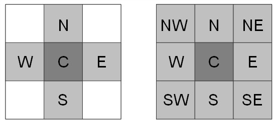
Fig. 11.1 Von Neumann neighbourhood definition (left) that considers the group of four cells in the four cardinal directions from the central one, and (right) the Moore method that includes the adjacent cells along diagonals.

To give physical meaning to the rule defining water interaction between two adjacent cells, the Darcy’s law is assumed. According to this, the water flux between central cell and, for example, northern cell, \(Q_{NC}\) [L³ T⁻¹], is calculated as:

(11.1)\[Q_{NC} = \frac{2T_{N}T_{C}}{T_{N} + T_{C}}\left( h_{N}^{t} - h_{C}^{t} \right)\]

where \(T_{N}\) and \(T_{C}\) represent, respectively, the transmissivity [L² T⁻¹] of northern cell and central cell, \(h_{N}^{t}\) and \(h_{C}^{t}\) represent, respectively, hydraulic head [L] of northern cell and central cell at previous time step, \(t\). The term \(\frac{2T_{N}T_{C}}{T_{N} + T_{C}}\) is the harmonic mean of transmissivity. It has been chosen because of its property to remove the impacts of large outliers by limiting the flux to the lower value of transmissivity. The flux is positive if entering the central cell.

The total flux entering the central cell is ( Fig. 11.2 ):

(11.2)\[Q_{C} = Q_{NC} + Q_{EC} + Q_{SC} + Q_{WC} + W_{C}\]

where \(W_{C}\) [L³ T⁻¹] is the volumetric flux representing sources (+) or sinks (-).

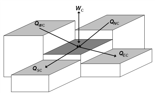
Fig. 11.2 Scheme for the calculation of water fluxes between the central cell and the four adjacent cells. \(W_{C}\) is the volumetric flux representing source (entering the cell) or sink (exiting the cell).

Hydraulic head at central cell is updated for the subsequent time, \(t + 1\), applying the discrete mass balance equation:

(11.3)\[h_{C}^{t + 1} = h_{C}^{t} + \frac{1}{S_{y}}\frac{Q_{C}}{\Delta s^{2}}\Delta t\]

where \(\Delta t\) [T] is the time step.

BOX 11.A Drawdown due to a constant pumping rate from a well

The numerical model was validated with respect to transient solution of head drawdown due to a constant pumping rate from a well. The first mathematical analysis was obtained by Theis (1935), under the assumptions that: (a) the aquifer is confined and compressible; (b) there is no source of recharge to aquifer; (c) water is released instantaneously from the aquifer as the head is lowered; (d) the well is fully penetrating.

The solution of unsteady distribution of drawdown is expressed by:

(11.4)\[s(r,t) = \frac{Q}{4\pi T} \cdot W(u)\]

with

(11.5)\[u = \frac{r_{}^{2} \cdot S_{y}}{4tT}\]

and

(11.6)\[W(u) = \int_{u}^{\infty}\frac{e^{- z}}{z}\]

where \(s\), is drawdown [L]; \(Q\), is the constant pumping rate [L³T⁻¹]; \(t\), time since pumping began [T]; \(r\), radial distance from the pumping well [L]. The integral expression is termed the well function. It is generally evaluated with analytical approximation. Barry et al. (2000) proposed a solution valid for all values of the argument of exponential integral. The Theis equation can be extended to describe flow in unconfined aquifers if the drawdown is small relative to the saturated thickness of the aquifer (Jacob, 1950).

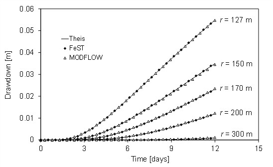
The domain was setup applying Dirichlet condition on the entire boundary with hydraulic head h = 50 m, as well as initial condition. A well with a constant pumping rate of 0.001 m³/s was placed in the central cell. The time step was set to 4000 s. Monitoring wells were placed along cardinal directions at a distance of 150, 200, 300 m from the pumping well. Two monitoring wells were placed on the 45 degrees direction at a distance of 127 and 170 m to investigate the eventuality that von Neumann neighbourhood could generate privileged directions. A further monitoring well was positioned at the cell adjacent to the boundary to verify if boundary condition could have influence on the cone of depression.

The following figure illustrates the depletion computed by the FeST model and MODFLOW-2000 compared to analytical solution for a 12 days duration after the beginning of the pumping. A very good fit can be observed in both monitoring wells along cardinal and diagonal direction.

Comparison between analytical (Theis) and numerical solution (FeST and MODFLOW) for head drawdown due to a constant pumping rate of 0.001 m³/s at distance r = 150, 200 and 300 m from the well along cardinal direction, and r = 127 and 170 m on the 45° direction.

11.2. River-aquifer interaction

Rivers contribute water to or drain water from the ground-water system, depending on the head gradient between the river and the ground-water regime. Quantification of stream/aquifer hydraulics is an important problem in the study of alluvial aquifers, and river base flow assessment.

In all cells adjacent to river network, river interconnection is simulated, which allows stream to gain or lose water. The stream stage is used to calculate the flux between the stream and the aquifer system, proportional to the head gradient between the river and the aquifer and a streambed conductance parameter. When the aquifer head is above the bottom of the streambed, model assumes that the discharge through the streambed is proportional to the difference in hydraulic head between the stream and the aquifer:

(11.7)\[Q = \frac{K_{sb}L\ W}{M}\left( h_{w} - h \right)\]

where \(Q\) is the discharge [L³T⁻¹] with a downward flux assumed positive, \(K_{sb}\) is the streambed hydraulic conductivity [LT⁻¹], \(L\) is the stream length [L], \(W\) is the stream width [L], \(M\) is the streambed thickness [L], \(h_{w}\) is the hydraulic head in the stream [L], and \(h\) is the hydraulic head in the aquifer [L]. If the aquifer head drops below the bottom of the streambed, the model assumes that the seepage flow is no longer proportional to the aquifer head and becomes dependent on the water level in the stream and the streambed thickness:

(11.8)\[Q = \frac{K_{sb}LW}{M}\left( H_{w} + M \right)\]

where \(H_{w}\) is the water level in the stream above the surface of the streambed [L]. At the beginning of each iteration, terms representing river seepage are added to the groundwater flow equation for each cell containing a river reach. Negative seepage occurs when river stage drops below aquifer head. Groundwater seepage is added to or subtracted from river flow accordingly.

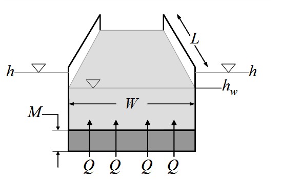
Fig. 11.3 Conceptual representation of river-aquifer interconnection: \(Q\) is the discharge, \(L\) is the stream length, \(W\) is the stream width, \(M\) is the streambed thickness, \(h_{w}\) is the hydraulic head in the stream, and \(h\) is the hydraulic head in the aquifer.

BOX 11.B Aquifer response to stream-stage variation

FeST capability to simulate the aquifer response to stream-stage variation is compared to the solution obtained by MODFLOW-2000.

The river interconnection was simulated using the RIVER package in MODFLOW-2000, which allows stream to gain or lose water. The stream stage is used to calculate the flux between the stream and the aquifer system, proportional to the head gradient between the river and the aquifer and a streambed conductance parameter, according to Equations (11.7) and (11.8) , as represented in ( Fig. 11.3 ).

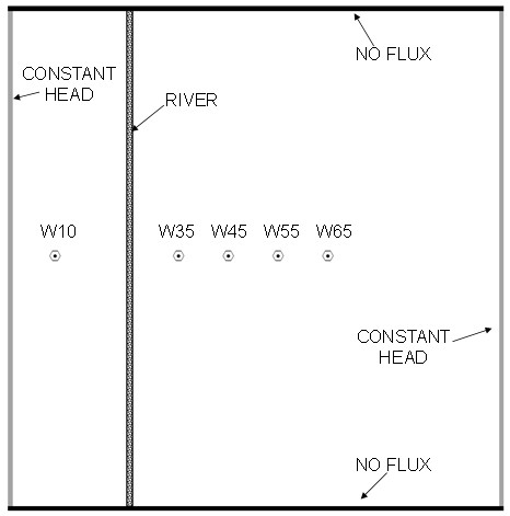
The domain was set up applying a constant head h = 50 m on the west and east boundaries, a Neumann type B condition on north and south boundaries, and an initial condition to perform the test. The time step was set to 4000 s. A river was placed with north-south direction at a distance of 250 m from the west boundary. River bottom was set at 46.5 m. Riverbed conductivity and thickness were 1·10⁻⁵ m/s and 0.5 m, respectively, and the width of the river was equal to 5 m. Monitoring wells were placed at a distance of 100, 350, 450, 550, and 650 m from the west boundary.

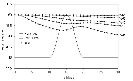
The simulation time was 30 days and the river stage was supposed to increase with a sinusoidal variation to a maximum of 50 m as reported in Figure 14 where the comparison between FeST and MODFLOW-2000 results is performed. A good agreement can be observed.

Scheme of the domain setup to perform the simulation of the aquifer response to stream-stage variation: location of river, boundary conditions and monitoring wells (W10, W35, W45, W55, and W65) are shown.

River stage variation and response of the water table at the five monitoringwells simulated by MODFLOW-2000 and FeST.

11.3. Boundary conditions

The final component of a CA model is the boundary condition that describes what happens at the outer cells of the lattice. The boundary conditions can be of Dirichlet or Neumann type (Kinzelbach, 1986). Dirichlet conditions specify the head h; Neumann conditions specify the flux, i.e., the head gradient \(\frac{\partial h}{\partial x}\) orthogonal to the boundary ( Fig. 11.4 ).

In Neumann type boundary cells, the subsurface flow coming from hydrological simulation is transformed into a flux entering unconfined aquifer along the border. Dirichlet type boundary condition cells are set along the border of the aquifer where piezometric head is considered constant in time.

In groundwater domain, percolation depurated from capillary rise computed by hydrological model is transformed into net recharge to groundwater storage.

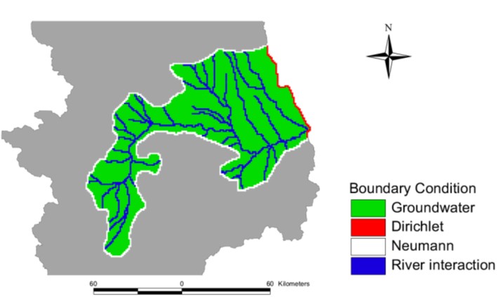
Fig. 11.4 Aquifer conceptual model: scheme of boundary conditions. In Neumann type boundary cells, the subsurface flow coming from hydrological simulation is transformed into a flux entering unconfined aquifer along the border. Dirichlet type boundary condition cells are set along the eastern border of the aquifer that continues downward into the Po valley.