2. Meteorological data

This section provides information about how meteorological data are processed before being used for hydrological simulation. Station measurements are interpolated according to one of the three available options, Thiessen polygons, inverse distance weighting, and Kriging methods. Station coordinates are converted to the spatial reference system of the simulation domain, before interpolation takes place. For considering effect of topography on meteorological data, some specific algorithms are, optionally, applied for interpolating solar radiation, air temperature, precipitation, and wind speed. Gridded data are converted to the proper reference system and spatially downscaled to the simulation grid resolution with nearest neighbour resampling method.

2.1. Spatial interpolation methods

2.1.1. Thiessen polygons

The Thiessen polygon method (Thiessen, 1911) is one of the simplest techniques, still widely used in hydrological studies, also referred to as the nearest neighbour method or Voronoi tessellation. It predicts the attributes of unsampled points based on those of the nearest sampled point. Polygons are drawn according to the distribution of the sampled data points, with one polygon per data point, which is then located in the centre of the polygon (Hartkamp et al., 1999). This method produces an abrupt transition between boundaries.

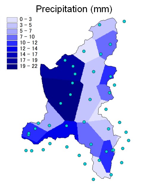
Fig. 2.1 Interpolation of precipitation (mm) acquired by raingauges (circles) with Thiessen polygon method in the Toce river basin, Italy.

2.1.2. Inverse distance weighting

The inverse distance weighting (IDW) is a deterministic estimation method whereby values at unsampled points are determined by a combination of values at known sampled points. Weighting of nearby points is strictly a function of distance (Shepard, 1968). The assumption is that values closer to the unsampled location are more representative of the value to be estimated. This method produces a gradual change of interpolated surface. The weight, \(\lambda\), of the \(i^{th}\) unsampled point is computed as:

(2.1)\[\lambda_{i} = \frac{\frac{1}{d_{i}^{p}}}{\sum_{i = 1}^{n}\frac{1}{d_{i}^{p}}}\]

where \(d_{i}\) is the distance from the known point to the unsampled point, \(n\) is the total number of known points used in interpolation and \(p\) is a positive real number, called the power parameter.

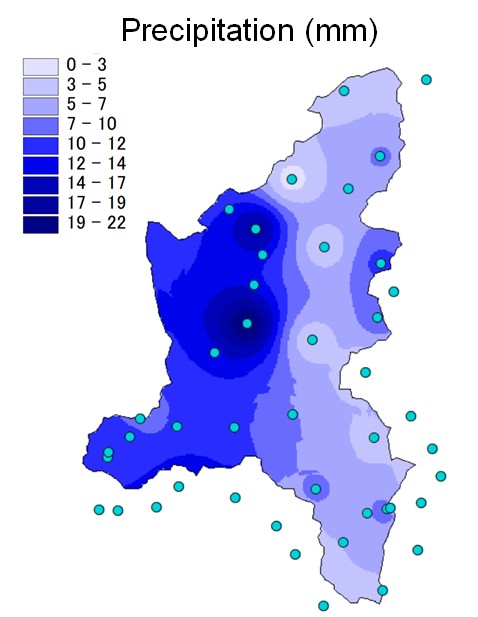
Fig. 2.2 Interpolation of precipitation (mm) acquired by raingauges (circles) with IDW method in the Toce river basin, Italy.

2.1.3. Kriging (ordinary)

The main assumption at the base of geostatistical methods is to consider variables of interest as random variables, and the observed reality as the result of random processes. The most popular geostatistical method is the Kriging method, which defines the interpolated value as a linear combination of weighted known values. The theoretical basis for the method was developed by the French mathematician Georges Matheron in 1960, based on the master’s thesis of Danie G. Krige, the pioneering engineer who developed the stochastic approach to compute the accuracy of the estimated gold concentration in mining engineering in the 1950s. Kriging is a weighted mean in which weights are chosen so that the error associated with the estimator is as small as possible. Weights depend on the position of the points used for the interpolation and on the covariance that is reflected in the variogram (Pari and Nofziger, 1987).

The most commonly used kriging method is the ordinary kriging, from now on pointed as OK. The aim of OK is to estimate the value of a random variable \(z(x)\) at a point \(x_{0}\) (so \(z\left( x_{0} \right)\) ), using data \(z\left( x_{i} \right)\) in the neighbourhood of the estimation location as reported in equation (2.2) where \(\lambda_{i}\) are the OK weights and \(n\) is the number of data closest to the location \(x_{0}\) to be estimated (Pellicone et al., 2018)

(2.2)\[z_{0}^{*}\ = z^{*}\left( x_{0} \right) = \sum_{i = 1}^{n}\lambda_{0_{i}}z\left( x_{i} \right) = \sum_{i = 1}^{n}\lambda_{0_{i}}z_{i}\]

In particular, \(\lambda_{i}\) values must be evaluated in order to obtain an unbiased estimation and to minimize the variance ( equation (2.5) ). By imposing that the interpolated value has to be unbiased we obtain that the weights sum must be equal to 1 ( equation (2.4) ).

(2.3)\[\in_{0}\ = \ z^{*}\left( x_{0} \right) - z\left( x_{0} \right) = \ z_{0}^{*} - z_{0}\]

(2.4)\[\overline{\in_{0}}\ = \ E\left\lbrack z_{0}^{*} - z_{0} \right\rbrack = 0\ z_{0}^{*} - z_{0} = > \ \sum_{i = 1}^{n}\lambda_{0_{i}} = 1\]

(2.5)\[Var\left( \in_{0} \right) = Var\left\lbrack z_{0}^{*} - z_{0} \right\rbrack = E\left\lbrack \left( z_{0}^{*} - z_{0} \right)^{2} \right\rbrack \rightarrow min\]

By substituting equation (2.2) in equation (2.5), and by taking into account the constraint expressed by equation (2.4), the following expression is obtained,

(2.6)\[Var\left( \in_{0} \right) = - \sum_{i = 1}^{n}{\sum_{j = 1}^{n}{\lambda_{0_{i}}\lambda_{0_{j}}\gamma\left( x_{i} - x_{j} \right)}} + 2\sum_{i = 1}^{n}{\lambda_{0_{i}}\gamma\left( x_{i} - x_{0} \right)}\]

where \(\gamma\) is the variogram, a growing monotone function representing the spatial correlation of points at increasing distance; it’s closely related to the covariance function and it’s defined by equation:

(2.7)\[\gamma(h) = \frac{1}{2}E\left\lbrack \left( z(x) - \ z(x + h) \right)^{2} \right\rbrack = \sigma_{z}^{2} - C(h)\]

where \(h\) is called lag and it represents the distance between two points \(x\) and \(x + h\), \(z\) is the value of the considered random variable measured in the two points, \(\sigma_{z}^{2}\) is the variance of the random variable \(z\) and \(C(h)\) is the covariance of \(( z(x), z(x + h) )\).

The variogram graph ( Fig. 2.3 ) shows on the horizontal axis the lag \(h\), on the vertical axis the variogram and it’s characterized by 3 parameters:

• sill (threshold): it’s the value of the variogram for which \(\gamma (h)\) becomes constant (\(C(h) ≈ 0\)), corresponding to uncorrelated observations of the variable \(z\) (asymptote of the variogram) (here, \(C_{0} + C_{1}\));

• range (or lenght): it’s the distance at which the observations are no longer correlated (it can be infinite or finite); usually is computed as the distance at which the 95% of the sill is reached;

• nugget: it’s the discontinuity visible at the origin and it represents variations of very small scale and/or measurement errors (here \(C_{0}\)).

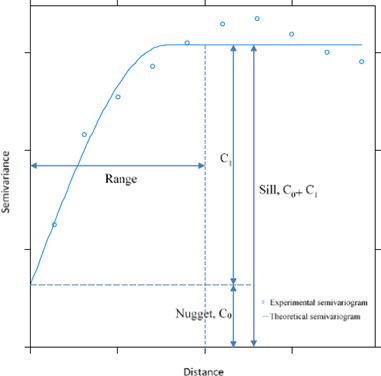
Fig. 2.3 Variogram graph.

So, before starting to use the OK method, it’s necessary to perform the variographic analysis, that means to compute an experimental variogram by using the available data, and then to fit a variogram model on the experimental one.

Several variogram models exist. Some of the most common are:

• Spherical:

(2.8)\[\begin{split}\gamma(h) = \left\{ \begin{array}{r} c\left( \frac{3h}{2a} - \frac{1}{2}\left( \frac{h}{a} \right)^{3} \right),\ \ \ \ \ \ \ \ \ h \leq a \\ \ \ \ \ \ \ \ \ \ \ \ \ \ \ \ \ \ c,\ \ \ \ \ \ \ \ \ \ \ \ \ \ \ \ \ \ \ \ \ \ h > a \\ \end{array} \right.\ \end{split}\]

• Exponential:

(2.9)\[\gamma(h) = c\left\{ 1 - exp( - \frac{h}{r}) \right\} \]

• Gaussian:

(2.10)\[\gamma(h) = c\left\{ 1 - exp( - \frac{h}{r}) \right\} \]

where \(c\) is the sill and \(a\) is the range.

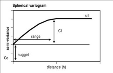
Fig. 2.4 Spherical semi-variogram model.

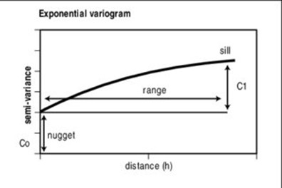
Fig. 2.5 Exponential semi-variogram model.

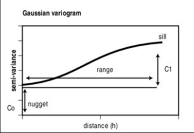
Fig. 2.6 Gaussian semi-variogram model.

The experimental variogram \(\widehat{\gamma}(h)\) is a discrete function of the lag \(h\) computed by using the following equation between pairs of points \([z(x_{i}), z(x_{i}+h)]\) at various distances, where \(n(h)\) is the number of data pairs for the specified lag vector \(h\).

(2.11)\[\widehat{\gamma}(h) = \frac{1}{2n(h)}\sum_{i = 1}^{n(h)}\left\lbrack z\left( x_{i} + h \right) - z\left( x_{i} \right) \right\rbrack^{2}\]

The procedure implemented in the FeST model implies that, firstly the semivariogram is generated from a given sample. The sample point pairs are ordered into even-width bin, separated by the euclidean distance of the point pairs. The semivariance in the bin is calculated by the Matheron estimator (equation (2.10)). If number of lags and lag max distance are not given they are automatically computed or set to default value, 15. The user can choose among spherical, exponential and gaussian semivariogram models or leave the program to automatically fit it to the best fitting model among the three, considering the nugget effect. Fitting algorithm is adapted from the VARFIT model by Pardo-Iguzquiza (1999). The VARFIT algorithm performs a nonlinear minimization of the weighed squared differences between the experimental variogram and the model.

(2.12)\[F(\theta) = \sum_{i = 1}^{NDIR}{\sum_{j = 1}^{NLAG(i)}{w(i,j)\left\lbrack \widehat{\gamma}(i,j) - \gamma(i,j;\theta) \right\rbrack^{2}}}\]

where NDIR is the number of directions. \(NLAG(i)\) is the number of lags in the \(i^{th}\) direction, \(\ \widehat{\gamma}(i,j)\) is the experimental variogram for the \(i^{th}\) direction and \(j^{th}\) lag, \(\gamma(i,j;\theta)\ \) is the variogram model with parameters vector \(\theta\).

By considering several directions in fitting the variogram, anisotropy can be accomplished. Indeed, variation can itself vary with direction. In this case the range, instead of being a constant, describes an ellipse in the plane of the lag. This is shown in Figure 5.13, where A is the maximum diameter of the ellipse, i.e. the range in the direction of greatest continuity (least change with separating distance), and B is the minimum diameter, perpendicular to the first, and is the range in the direction of least continuity (greatest change with separating distance). The angle \(\varphi\) is the direction in which the continuity is greatest.

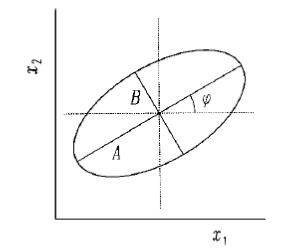
Fig. 2.7 A representation of geometric anisotropy in which the ellipse describes the range of a spherical variogram in two dimensions. The diameter A is the maximum range of the model, B is the minimum range, and \(\varphi\) is the direction of the maximum range (adapted from Webster and Oliver (2007).

When aniisotropy option is activated by the user, the FeST computes the empirical variogram in the four directions:

• East-South (0°)

• NorthEast-SouthWest (45°)

• North-Sout (90°)

• NorthWest-SoutEast (315°)

The weighting function, \(w\) is computed as:

(2.13)\[w(i,j) = N(i,j){\lbrack\gamma(i,j);\theta\rbrack}^{- 2}\]

where \(N (i, j)\) is the number of data pairs used to obtain the estimate \(\widehat{\gamma}(i,j).\)

The weighting function has an important statistical attraction. The uncertainty of the variogram estimate \(\ \widehat{\gamma}(i,j)\) is (Cressie, 1985):

(2.14)\[Var\lbrack\widehat{\gamma}(i,j)\rbrack \approx {\lbrack\gamma(h)\rbrack}^{2}/N(h)\]

where \(Var\lbrack{X}\rbrack\) is the variance of the random variable \(X\), \(\gamma(h)\) is the true variogram and \(N(h)\) is the number of data pairs used in the estimation of i \(\widehat{\gamma}(i,j)\).

Then it is logical to weigh each estimate \(\ \widehat{\gamma}(i,j)\) by the inverse of its estimation variance. These weights (the inverse of the estimation variance) are optimal when the different estimates are independent (Hoel, 1984). This is not the case for the experimental variogram where the different estimates (\(\widehat{\gamma}(i,j)\) for different \(h\)) are correlated; in this situation a generalized least squares method would be more appropriate; but the weighted least squares represent a good compromise of statistical efficiency and computability (Cressie, 1985). This weighting function seems to give good results in practice (Gotway, 1991; Zimmerman and Zimmerman, 1991).

VARFIT uses a non-linear minimisation method that does not require (explicit) initial values for the parameters in order to initialise the minimisation algorithm. Jian et al. (1996) report problems with convergence if the initial guess is poor. Solution is found with the simplex method of function minimization of Nelder and Mead (1965). This ingenious method is efficient for non-linear minimization in a multiparameter space but is still easy to program and only requires evaluations of the objective function. The program stops the iterations whenever one of the two following criteria is reached:

1. Convergence is reached

2. The maximum number of iterations is reached.

3. The best fitted semivariogram model is used

The best fitted semivariogram model is used to interpolate a regular grid of data. Code is adapted from the Geostats program written by Luke Spadavecchia, Biosphere Atmosphere Modelling Group, University of Edinburgh, November 2006. A number of closest points are used to build the covariance matrix used to predict value at location where value is unknown. Matrix inversion uses the the Gauss-Jordan method. An n*2,n work array is assembled, with the array of interest on the left half, and the identity matrix on the right half. A check is made to ensure the matrix is invertable, and the matrix inverse is returned, providing the matrix is not singular. The matrix is invertible if, after pivoting and row reduction, the identity matrix shifts to the left half of the work array.

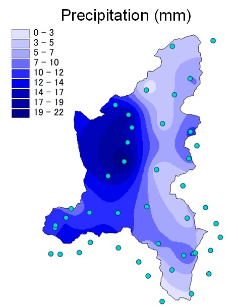
Fig. 2.8 Interpolation of precipitation (mm) acquired by raingauges (circles) with OK method in the Toce river basin, Italy.

BOX 2.A Reliability of methods to interpolate precipitation

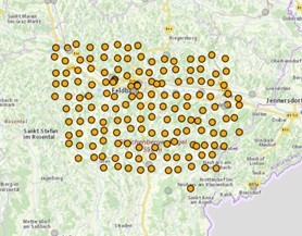
Three techniques – Thiessen, IDW, and OK – are evaluated for interpolation of precipitation data available through the WegenerNet data portal (https://wegenernet.org/).

The WegenerNet site is located in the South-East of Austria, in the federal state of Stiria, close to Feldbach, in the Raab river’s valley. It’s a hilly area, with a range of elevation that goes from 257 to 609 m a:s:l. The University of Graz installed a net of 150 weather stations placed on a regular grid with a density of one station per 2 km² and 5-min interval data acquisition. Data are available since Jan 1, 2007. In this analysis data of 2016 were used.

Map of available stations in the WegenerNet data portal https://wegenernet.org

In order to evaluate and compare the performance of interpolation methods, the leave-one-out statistical method is adopted. It checks the compatibility between the input data and the model by removing once at time each data point from the dataset and by using information from remaining data-points to predict the variable value in the point temporarily from the dataset. Performance indexes are computed at every time step (hour) and averaged over the whole period (2016).

Results show that Thiessen is the worst method, while IDW and OK have comparable performances.

	RMSE	NMRSE	NSE	PCC
Thiessen	0.390	1.022	0.052	0.527
IDW	0.336	0.825	0.412	0.623
OK exponential	0.300	0.788	0.442	0.618

Performance results in terms of root mean square error (RMSE) normalised RMSE (NRMSE), the coefficient of determination (NSE), and Pearson correlation coefficient (PCC) for Thiessen, IDW and OK with exponential semivariogram.

2.2. Net radiation over complex topography

When the direct and diffuse shortwave (solar) radiation reach the land surface, some of this radiation is reflected by the surface ( Fig. 2.9). The fraction of the incoming shortwave radiation that is reflected by the surface is called the albedo. In addition to the shortwave radiation, we need to account for the longwave radiation at the land surface. Land surface emits longwave radiation to the atmosphere. But, we should not overlook the fact that the atmosphere emits longwave radiation both upward into space and downward toward the Earth’s surface. The magnitude of this downward longwave radiation depends on the temperature and emissivity of the atmosphere. The presence of clouds significantly increases the emissivity of the atmosphere. The amount of water vapor in the atmosphere also has a strong effect on the atmospheric emissivity, with higher emissivity values for more humid conditions.

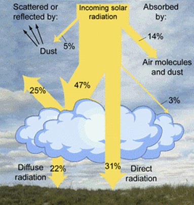
Fig. 2.9 Partitioning of solar radiation by the atmosphere. Source: (https://open.library.okstate.edu/rainorshine/chapter/11-3-net-radiation/)

Net radiation is simply the sum of all incoming and outgoing radiation fluxes at the land surface. Mathematically, net radiation, \(R_{n}\), is given by:

(2.15)\[R_{n} = S_{in} - S_{out} + L_{in} - L_{out}\]

with

(2.16)\[S_{in} - S_{out} = (1 - r)S_{in}\]

(2.17)\[L_{in} - L_{out} = {(1 - r)R_{ld} - R}_{lu}\]

where \(S\) denotes shortwave radiation, \(L\) longwave radiation, subscripts \(in\) and \(out\) denotes input and output to and from the ground, respectively, \(r\) is albedo, \(R_{ld}\) is longwave radiation emitted from ground, and \(R_{lu}\) is longwave radiation emitted from atmosphere.

2.2.1. Shortwave radiation

The radiation components can be highly modified by local and surrounding topography. In fact the topography affects the radiation field in three ways ( Fig. 2.10):

1. modulating the actual energy flux according to the relative position of the ground surface with respect to the sun;

2. reducing radiation because of shadowing effect of the higher crests of mountains;

3. increasing net radiation by the fraction reflected from neighbouring terrains.

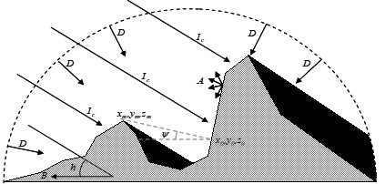
Fig. 2.10 Shortwave radiation affected by topography

When option is set by user to account for topography effect, the FeST model adjusts incoming shortwave radiation before computing net radiation.

The incident short wave radiation can be expressed as:

(2.18)\[S_{in} = Q_{a} + DF + A\]

where \(Q_{a}\) is direct radiation component affected by topographic characteristics, such as slope and aspect, \(DF\) is the actual scattered radiation from sky, \(A\) is the radiation reflected from neighbour terrain.

The position of the Sun in the sky is expressed in terms of the solar altitude and the solar azimuth. The height of the Sun, the elevation of the Sun, is usually given in terms of the solar altitude \(h\). This is the angular distance between the Sun’s rays and the horizon (Gates, 1980). And the solar azimuth, \(B\), is the horizontal angle with respect to north (Oke, 1987).

(2.19)\[\sin(h) = \sin(\phi)\sin(d) + \cos(\phi)\cos(d)\cos(\eta)\]

(2.20)\[\cos(B) = \left\lbrack \sin(d)\cos(\phi) - \cos(d)\sin(\phi)\cos(\eta) \right\rbrack/\cos(h)\]

where \(\phi\) is the local latitude and \(\eta\) is the solar hour angle (Iqbal, 1983)

(2.21)\[\eta = 15(t - 12)\]

\(t\) is the hour of day.

Solar declination, \(d\), is the angle between the Earth–Sun line and the equatorial plane (Iqbal, 1983).

(2.22)\[\begin{split}d = \left( \begin{aligned} & 0.006918 - 0.399912\cos(\Gamma) + 0.070257\sin(\Gamma) - 0.006758\cos(2\Gamma) \\ & + 0.000907\sin(2\Gamma) - 0.002697\cos(3\Gamma) + 0.00148\sin(3\Gamma) \\ \end{aligned} \right)\end{split}\]

\(\Gamma\) is the day angle:

(2.23)\[\Gamma = \frac{2\pi(J - 1)}{365}\]

where \(J\) is the Julian day, representing number of days after 1 January.

In clear sky conditions, the incoming solar radiation reaching the ground in the normal direction is:

(2.24)\[I_{c} = I_{0}\exp{\left\lbrack \frac{- s}{\sin(h)} \right\rbrack\sin(h)}\]

where \(I_{0}\) is direct solar irradiance at the top of the atmosphere (solar constant =1367 W/m²), \(s\) is the atmosphere optical depth (Kreider and Kreith, 1978):

(2.25)\[s = s_{0}\frac{P_{z}}{P_{0}}\]

with \(s_{0}\) the atmospheric optical depth at sea level:

(2.26)\[s_{o} = \sqrt{1229 + \left( 614\ \sin(h) \right)^{2}} - 614\ \sin(h)\]

\(\frac{P_{z}}{P_{0}}\) is a correction factor that takes into account the difference in atmospheric pressure between sea level (\(P_{0}\)) and actual elevation (\(P_{z}\)):

(2.27)\[P_{h}/P_{o} = \left( (288 - 0.0065\ z)/288 \right)^{5.256}\]

where \(z\) is the altitude above sea level.

The scattered radiation for clear sky condition, \(D\), is:

(2.28)\[D = k_{b}\left( I_{0}\sin(h) - I_{c} \right)\]

where \(k_{b}\) varies from 0.2 to 0.6 according to the sky brightness (set to 0.4 in the FeST model).

In clear sky condition, the theoretical radiation observed at the ground level, R^(*), is expressed by:

(2.29)\[R^{*} = I_{c} + D\]

The presence of clouds or natural obstacles reduces the direct radiation \(I_{c}\) and modifies the scattered one so that \(R^{*}\) can be reduced to a minimum fraction, \(p\), of \(R^{*}\) (usually \(p = 0.22\) is referred to a transmissivity coefficient for 8/8 stratocumulus cloud cover (Male and Granger, 1981). When the observed radiation is less or equal to \(pR^{*}\), radiation is considered totally scattered (sky totally covered with clouds). Otherwise, the fraction of scattered radiation, \(K_{t}\), is computed as (Ranzi, 1989):

(2.30)\[K_{t} = \frac{R^{*} - Rs}{\left\lbrack (1 - p)R^{*} \right\rbrack}\]

Finally, the component of the actual scattered radiation, \(DF\), can be computed as:

(2.31)\[DF = min\left\lbrack R_{s},D\left( 1 - K_{t} \right) + R_{s}K_{t} \right\rbrack\]

and direct radiation component, \(Q\), as:

(2.32)\[Q = R_{s} - DF\]

Direct radiation component, \(Q\), is affected by topographic characteristics, such as slope, \(\alpha\), and aspect, \(E\). Actual direct radiation, \(Q_{a}\), is related to the sun elevation as:

(2.33)\[Q_{a} = \frac{Q\ cos(C)}{\sin(h)}\]

The angle ( Fig. 2.10 ) between the sunbeam direction and the perpendicular to the ground is evaluated with:

(2.34)\[\cos(C) = cos(h)\sin(\alpha)\cos(B - E) + sin(h)\cos(\alpha)\]

The radiation reflected from neighbour terrain is:

(2.35)\[A = Q_{a} \cdot r \cdot (1 - f_{\alpha})\]

where \(f_{\alpha} = 1 - \alpha/180{^\circ}\).

A module taking into account the shadow effect induced by topography was developed. Firstly, the algorithm determines for each cell the sky view angle, that is the maximum horizontal viewing angle of terrain obstruction in a given direction based on the elevations of traversed cells and their distances to the viewing point ( Fig. 2.11 ) (Zhang et al., 2017). The sky view angle is computed along 16 directions equally spaced by 22.5 degrees ( Fig. 2.12 ). To select the traversed cells by the solar beam direction, a finite number of points is considered, starting from the centre of the initial cell (viewing point) ( Fig. 2.13 ). The coordinate of points is computed by summing the increment along east direction, \(\mathrm{\Delta}x\), and north direction, \(\mathrm{\Delta}y\), as:

(2.36)\[\mathrm{\Delta}x = \delta\ sin(B)\]

(2.37)\[\mathrm{\Delta}y = \delta\ cos(B)\]

where \(B\) is the azimuth and \(\delta\) is the half of domain cell size.

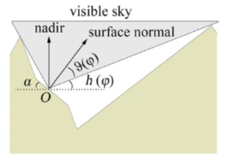
Fig. 2.11 A cross section of a valley to sketch the visible sky area from a slope in the valley. h(φ) is the maximum horizontal viewing angle of terrain obstruction in azimuth φ. ϑ(φ) is the zenith angle to the slope normal of terrain horizon on a sloped coordinate system in azimuth φ. Adapted from Zhang et al., 2017.

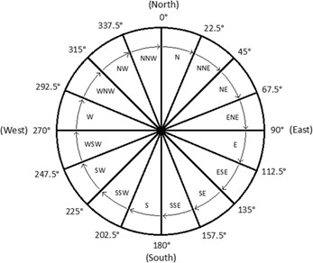
Fig. 2.12 The sixteen directions along which shy view angle is computed for each cell: (0.0, 22.5, 45.0, 67.5, 90.0, 112.5, 135.0, 157.5, 180.0, 202.5, 225.0, 247.5, 270.0, 292.5, 315.0, 337.5 degree)

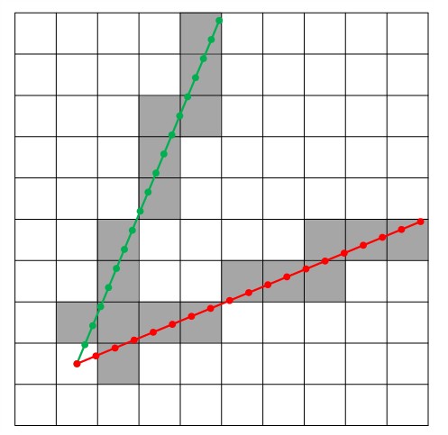
Fig. 2.13 Traversed cells from the viewing point for 22.5° azimuth direction (green line), and 67.5° azimuth direction (red line). Points mark position of points computed as successive increment from the viewing point.

The angle, \(\omega\), between the point with maximum elevation in the direction of the solar beam, denoted by coordinates \(x_{m}\), \(y_{m}\), \(z_{m}\) , and the examined cell, denoted by coordinated \(x_{0}\), \(y_{0}\), \(z_{0}\) ( Fig. 2.10 ):

(2.38)\[\omega = arctg\left( \frac{z_{m} - z_{0}}{d_{m0}} \right)\]

where \(z_{m}\) and \(z_{0}\) are terrain elevation (retrieved from digital elevation model) of the point with maximum elevation, \(m\), and the viewing point, \(0\), respectively, and \(d_{m0}\) is the distance between point \(m\) and point \(0\).

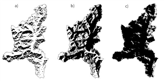
Fig. 2.14 Shadow maps on the Toce river basin, Italy, for three different times: a) 2000-02-01T12:00:00+00:00, azimuth 180°, sun elevation 28°; b) 2000-02-01T08:00:00+00:00, azimuth 123°, sun elevation 7.6°; c) 2000-02-01T16:00:00+00:00, azimuth 233°, sun elevation 3°.

At every simulation time step, the current sun elevation and azimuth are computed as a function of the hour of day and day of year, and the closest direction out of the 16 ones is selectes. A map of shadowed pixels is computed comparing \(\omega\) with sun elevation in each cell. If \(\omega\) is higher than the sun elevation, the cell is shadowed and the incident short wave radiation is constituted by scattered and reflexed components only:

(2.39)\[R_{s} = DF + A\]

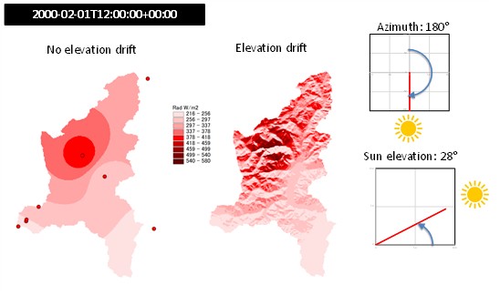
Fig. 2.15 Shortwave radiation at 12:00 of 2000-02-01 on the Toce river, Italy, interpolated with inverse distance weighting without drift (left) and with elevation drift (right). Circles show stations where solar radiation was measured.

2.2.2. Longwave radiation

Bodies at terrestrial temperatures emit radiation with typically long wavelengths around 10 \(\mu m\) and in any case not exceeding 100 \(\mu m\).

Although good instruments have become available for the measurement of longwave radiation, the measurement of this type of radiation is not simple and is rarely done; one reason for this is that any measuring instrument emits radiation of similar wavelengths and intensities to those it is supposed to measure.

To overcome the lack or the scarcity of longwave radiation measurements, it is necessary to estimate these data from proxy information. For this purpose, it is convenient to distinguish between long-wave radiation emitted by the earth’s surface \(R_{ld}\) and long-wave radiation emitted by the atmosphere \(R_{lu}\).

From the Stefan-Boltzmann equation, longwave radiation, \(R_{l}\) , can be written as:

(2.40)\[R_{l} = \xi_{s}\ \sigma\ (T_{s})^{4}\]

where:

\(\xi_{s}\) is emissivity of body surface

\(\sigma\) is the Stefan-Boltzmann constant ( 5.67 10⁻⁸ Wm⁻²K⁻⁴ )

\(T_{s}\) is the body surface temperature (K)

The Stefan-Boltzmann equation requires the temperature of the body’s surface, a measure that is rarely available. Using the air temperature as alternative to surface body temperature can lead to a non-negligible error.

Alternatively the long-wave radiation can be estimate without measuring the surface temperature with an expression like (Wales-Smith, 1980):

(2.41)\[R_{ld} - R_{\ln} = - \sigma\ \left( T_{a}\ + 273.15 \right)^{4}\ \left( 0.56 - 0.079\sqrt{e_{a}} \right)\ (0.1 + 0.9\ cl)\]

where

\(T_{a}\ \) is the air temperature (degree Celsius)

\(e_{a}\) is the actual vapor pressure (Kpa), computed as:

(2.42)\[e_{a} = e_{s}(RH/100)\]

where \(RH\) (%) is the air relative humidity and \(e_{s}\) (Kpa) is the sature vapor pressure computed as a function of air temperature:

(2.43)\[e_{s} = 0.6108\ exp\ \left( \frac{17.27\ T_{a}\ }{T_{a} + 237.3} \right)\]

\(cl\) is the shadow factor computed as the complement to clearness factor, \(k_{t}\) (Liu and Jordan, 1960):

(2.44)\[cl = 1 - K_{t}\]

2.3. Air temperature with lapse rate

Air temperature is an important input to a variety of spatially distributed hydrological and ecological models. These models use air temperature to drive processes such as evapotranspiration, snowmelt, soil decomposition, and plant productivity (Dodson and Marks, 1997). Since most near-surface air temperature data are collected at irregularly spaced point locations rather than over continuous surfaces, the point-based temperatures must be accurately distributed over the landscape in order to be useful in spatially distributed modeling.

In mountainous terrain, the strong relationship between temperature and elevation precludes a simple interpolation of point-based temperature observations. Unless the effect of elevation on temperature is explicitly accounted for, an interpolation of temperature can produce grossly inaccurate results.

An additional problem with point-based temperature data is that the locations of meteorological stations tend to be biased toward lower elevations. Highelevation regions are represented poorly by the spatial distribution of most meteorological station networks (Robeson 1995).

The main difficulty in accurately interpolating temperature data in mountainous terrain is the effect of elevation on temperature. Mountains, acting as physical barriers, force air to move vertically, a process called orographic uplift. When an air parcel rises, it expands and cools. If no heat is exchanged with the outside system, this cooling is termed adiabatic. The rate at which air cools with elevation change, the lapse rate, varies from about -9.8°C km⁻¹ for dry air (the dry adiabatic lapse rate) to about -4.0°C km⁻¹ for very warm saturated air (the saturated adiabatic lapse rate) (Barry & Chorley 1987, p. 76). The lapse rate is seldom purely adiabatic due to outside heat exchange caused by radiational heating or cooling at the surface, horizontal mixing (advection) of air masses, and evaporation or condensation of moisture. The actual lapse rate at a given place and time is termed the environmental lapse rate. A typical value used for the global mean environmental lapse rate is -6.5°C km⁻¹ (Barry & Chorley 1987, p. 56).

The FeST model implements an interpolation algorithm to account for air temperature vertical lapse rate ( Fig. 2.16 ):

1. air temperature, \(T_{m}\), measured at elevation \(z_{m}\), is transformed to air temperature, \(T_{r}\) on a reference elevation, \(z_{r}\), keeping into account a fixed thermal lapse rate, \(\gamma\)

(2.45)\[T_{r} = T_{m} + \ \left( z_{r} - z_{m} \right)\ \gamma\]

2. data at reference elevation are interpolated using one of the methods implemented (Thiessen, IDW , OK) to fill in all cells of the simulated domain

3. in each cell of the simulation domain, air temperature at reference elevation is transformed back to air temperature, \(T_{g}\) , at elevation retrieved from digital elevation model, \(z_{dem}\), keeping into account a fixed thermal lapse rate

(2.46)\[T_{g} = T_{r} - \ \left( z_{r} - z_{dem} \right)\ \gamma\]

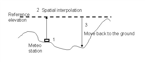
Fig. 2.16 Schematic of the air temperature interpolation considering a vertical lapse rate and elevation drift.

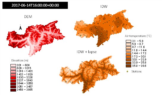
Fig. 2.17 Air temperature at 16:00 of 2017-06-14 on the Bolzano province, Italy, interpolated with inverse distance weighting without drift (IDW) and with elevation drift with lapse rate = -6.5 °C/km (IDW+lapse). Digital elevation model on the left.

Air temperature vertical lapse rate is assigned as a constant value. It can be assigned as a fixed scalar constant in time and space for the whole domain or as a raster map that may vary with time (by assigning a netCDF multidimensional map).

Optionally the lapse rate can be automatically computed at every simulation time step by a linear regression between the vector of measured air temperature data and vector of station elevation.

(2.47)\[\gamma = \frac{\sum_{i = 1}^{n}{\left( z_{m}^{i} - \overline{z_{m}} \right)\ \left( T_{m}^{i} - \overline{T_{m}} \right)\ }}{\sum_{i = 1}^{n}\left( z_{m}^{i} - \overline{z_{m}} \right)^{2}}\]

where \(n\) is the total number of available stations, and the upper line denotes average operator.

While air temperature lapse rate is computed, the square of the correlation coefficient, \(R^{2}\), is computed as well

(2.48)\[R^{2} = \frac{\left\lbrack n\sum_{i = 1}^{n}{\left( z_{m}^{i}\ T_{m}^{i} \right) - \sum_{i = 1}^{n}{\left( z_{m}^{i}\ \right)\ \ \sum_{i = 1}^{n}\left( T_{m}^{i}\ \right)}} \right\rbrack^{2}}{\left\{ n\sum_{i = 1}^{n}\left( z_{m}^{i} \right)^{2} - \left\lbrack \sum_{i = 1}^{n}\left( z_{m}^{i} \right) \right\rbrack^{2} \right\}\ \left\{ n\sum_{i = 1}^{n}\left( T_{m}^{i} \right)^{2} - \left\lbrack \sum_{i = 1}^{n}\left( T_{m}^{i} \right) \right\rbrack^{2} \right\}}\]

A minimum value of \(R^{2}\) can be set so that when actual value is below the threshold value, a fixed lapse rate value is used to interpolate air temperature. The following figure shows air temperature observations on the Bolzano province, Italy, plotted against station elevation, for two time step. The example on the left is of a time step where observations are strongly linearly correlated to elevation. The example on the right is of a time step where the correlation is very weak, due to thermal inversion phenomena very frequent in Alpine region during winter.

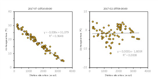
Fig. 2.18 Air temperature observations on the Bolzano province, Italy, plotted against station elevation, for two time step. Dotted line shows regression line. Linear regression equation and R2 metric are shown. The example on the left is of a time step where observations are strongly linearly correlated to elevation. The example on the right is of a time step where the correlation is very weak, due to thermal inversion phenomena very frequent in Alpine region during winter.

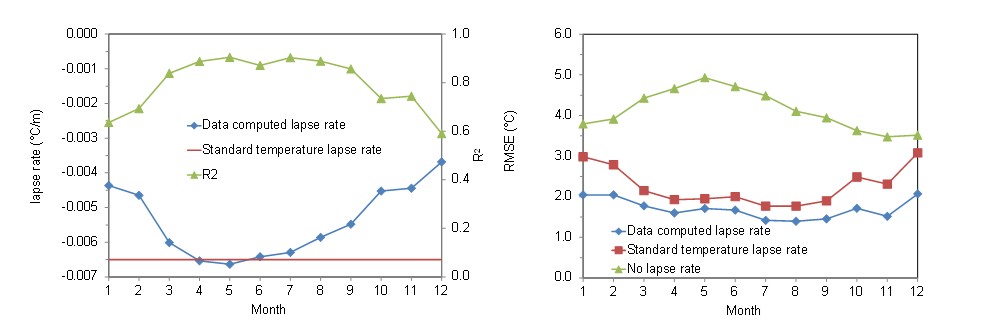
BOX 2.B Using lapse rate improves temperature interpolation

To verify the effect of the temperature lapse rate on the interpolation of the temperature data, a jackknife cross validation was applied considering the temperature measurements from 2016 to 2019 in the Bolzano province, Italy. At each hour, in turn, the data measured at a station was removed and the remaining measurements were interpolated to reconstruct the removed data, iteratively for all the available stations. For each hour the root mean square error was calculated between the observed data and those reconstructed with interpolation. The procedure was repeated considering: interpolation without lapse rate, interpolation with standard lapse rate (-0.0065 °C m⁻¹), and interpolation with lapse rate updated hourly from the linear regression of the observed data with respect to the altitude. Results are shown in the two figures on a monthly scale. It is noted that only in the period April-July the lapse rate calculated from data is comparable to the standard gradient, while the value of the calculated lapse rate decreases (in absolute value) significantly in the remaining months of the year with a minimum in December equal to - 0.0037 °C m⁻¹. The value of R² of the linear regression is relatively high (> 0.8) in the period between March and September, while it decreases in the rest of the year, due to the thermal inversion phenomenon, frequently occurring in autumn and winter, which causes a significant deviation from the linear trend of temperature with altitude. Figure (right) shows the monthly average results of the cross validation. We note how the interpolation that updates the lapse rate at each step shows a lower error in all months compared to considering the standard lapse rate or not considering a lapse rate in the interpolation.

Monthly air temperature lapse rate computed from linear regression of observations and related R2 compared to standard lapse rate (left), and monthly average root mean square error (RMSE) re-sulting from interpolation jackknife cross validation considering no lapse rate, standard lapse rate and lapse rate computed from data (right).

2.4. Precipitation with lapse rate

There is generally a limited number of rain gauges at high elevations due to the difficulties of installing and maintaining them. Even when there are stations, the precipitation measurement is often affected by significant errors, especially in the winter period caused by the presence of wind and by the malfunctioning of the heating system for snowfall melting. Precipitation in the Alps generally follows an increasing trend with elevation. Reconstructing a precipitation field considering only the measurements available at lower altitudes leads to an underestimation of the total precipitation volume (Avanzi et al., 2021). It is therefore crucial to evaluate the precipitation lapse rate to be used in spatial interpolation, including the measurements at the highest elevations (Corbari et al., 2022).

The FeST model implements an interpolation algorithm to account for precipitation vertical lapse rate that follows the same approach implemented for air temperature ( Fig. 2.16 ):

1. Precipitation, \(P_{m}\) (mm), measured at elevation \(z_{m}\) (m), is transformed to precipitation, \(P_{r}\) (mm) on a reference elevation, \(z_{r}\) (m), keeping into account a lapse rate, \(\gamma\) (mm/h/m), integrated over a time step, \(\mathrm{\Delta}t\) (h)

(2.49)\[P_{r} = P_{m} + \ \left( z_{r} - z_{m} \right)\ \gamma\ \mathrm{\Delta}t\]

2. data at reference elevation are interpolated using one of the methods implemented (Thiessen, IDW, OK) to fill in all cells of the simulated domain

3. in each cell of the simulation domain, precipitation at reference elevation is transformed back to precipitation, \(P_{g}\) , at elevation retrieved from digital elevation model, \(z_{dem}\), keeping into account the lapse rate integrated in the time step, \(\mathrm{\Delta}t\) (h)

(2.50)\[P_{g} = P_{r} - \ \left( z_{r} - z_{dem} \right)\ \gamma\ \mathrm{\Delta}t\]

Lapse rate can be assigned as a fixed scalar for the whole domain or as a raster map that may vary with time (by assigning a netCdf multidimensional map).

2.5. Wind speed over complex topography

Wind speed data are fundamental for evapotranspiration assessment in hydrological studies (Ravazzani et al., 2012). For application to large river basins, characterized by a limited number of available wind observation sites, data interpolation becomes necessary to estimate wind spatial variability (Cheng and Georgakakos, 2011). However, in complex topography areas, interpolation is made difficult because of spatial variation in wind velocity caused by slopes, canyons or valleys, and of the sheltering and diverting effects of terrain (Ryan, 1977; Rotach et al., 2015). Proposed methods for the wind field interpolation can be summarized as (Liston and Sturm, 1998):

1. applying a physically based numerical weather prediction model which satisfies all relevant momentum and continuity equations (Ercolani et al., 2015);

2. applying an atmospheric model in which only mass continuity is satisfied (Wagenbrenner et al., 2016);

3. interpolating wind-speed and direction observations in conjunction with empirical wind-topography relationships (Ryan, 1977).

Numerical weather prediction models have been run successfully for specific test cases that implies specialized model configurations and requires technical expertise and access to computing resources (Helbig et al., 2017).

Mass conserving models have been applied to small scale high spatial resolution domain and, even though less demanding than numerical weather models, they still require substantial resources when applied to larger scales (Forthofer et al., 2014).

For long-run simulations of hydrological processes in large river basins, simple empirical models are preferable in order to limit simulation time (Ravazzani et al., 2014).

In FeST model two options are implemented to constrain wind speed interpolation to topography:

• The MicroMet model by Liston and Elder (2006);

• The method presented by González-Longatt et al. (2015).

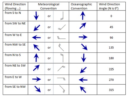
BOX 2.C Convention for wind speed direction

Meteorologists and oceanographers describe the flow of wind differently. Oceanographers prefer to describe wind in terms of the “direction of mass flow” or in other words the direction towards which the wind is blowing. In the oceanographic convention, wind flowing from the south to the north is symbolized by an arrow pointing north. Meteorologists (and hydrologists) use an arrow or a special symbol called a wind barb to show the direction from which the wind is blowing. The head of the arrow or wind barb points in the direction from which the wind is blowing. In the meteorological convention, a wind blowing from west to east is symbolized by an arrow pointing west.

Meteorological and oceanographic conventions to display wind direction. https://www.esri.com/arcgis-blog/products/product/analytics/displaying-speed-and-direction-symbology-from-u-and-v-vectors/

2.5.1. The MicroMet model

Observed values of wind speed \(W\) (m s⁻¹) and direction \(\theta\) are first converted into zonal \(u\) (m s⁻¹) and meridional \(v\) (m s⁻¹) wind components using:

(2.51)\[u = - W\sin\theta\]

(2.52)\[v = - W\cos\theta\]

Then, \(u\) and \(v\) components are independently interpolated to a regular grid using the IDW. The resulting values are converted back to wind speed using:

(2.53)\[W = \sqrt{u^{2} + v^{2}}\]

These gridded values are then modified to account for topographic variations, multiplying by an empirically based weighting factor, \(W_{w}\),

(2.54)\[W_{w} = 1 + \gamma_{s}\Omega_{s} + \gamma_{c}\Omega_{c}\]

where \(\Omega_{c}\) is the topographic curvature:

where \(\Omega_{s}\) is the topographic slope in the direction of the wind, \(\Omega_{c}\) is the topographic curvature, and \(\gamma_{s}\) and \(\gamma_{c}\) are positive constants which weight the relative influence of \(\Omega_{s}\) and \(\Omega_{c}\) on modifying the wind speed.

The curvature, \(\Omega_{c}\), is computed at each model grid cell by first defining a curvature length scale or radius, \(\mathbf{\eta}\) (m), that defines the topographic length scale to be used in the curvature calculation. This length scale is equal to approximately half the wavelength of the topographic features within the domain (e.g., the distance from a typical ridge to the nearest valley). Default value used by the FeST model for length scale is 5000 m.

For each model grid cell, the curvature is calculated by taking the difference between that grid cell elevation, and the average elevations of the two opposite grid cells a length scale distance from that grid cell. This difference is calculated for each of the opposite directions S–N, W–E, SW–NE, and NW–SE from the main grid cell (effectively obtaining a curvature for each of the four direction lines), and the resulting four values are averaged to obtain the curvature. Thus

(2.55)\[\begin{split}\mathbf{\Omega}_{\mathbf{c}}\mathbf{=}\frac{\mathbf{1}}{\mathbf{4}}\left\lbrack \begin{array}{r} \frac{\mathbf{z}\mathbf{-}\frac{\mathbf{1}}{\mathbf{2}\left( \mathbf{z}_{\mathbf{W}}\mathbf{+}\mathbf{z}_{\mathbf{E}} \right)}}{\mathbf{2}\mathbf{\eta}}\mathbf{+}\frac{\mathbf{z}\mathbf{-}\frac{\mathbf{1}}{\mathbf{2}\left( \mathbf{z}_{\mathbf{S}}\mathbf{+}\mathbf{z}_{\mathbf{N}} \right)}}{\mathbf{2}\mathbf{\eta}}\mathbf{+} \frac{\mathbf{z}\mathbf{-}\frac{\mathbf{1}}{\mathbf{2}\left( \mathbf{z}_{\mathbf{SW}}\mathbf{+}\mathbf{z}_{\mathbf{NE}} \right)}}{\mathbf{2}\sqrt{\mathbf{2}\mathbf{\eta}}}\mathbf{+}\frac{\mathbf{z}\mathbf{-}\frac{\mathbf{1}}{\mathbf{2}\left( \mathbf{z}_{\mathbf{NW}}\mathbf{+}\mathbf{z}_{\mathbf{SE}} \right)}}{\mathbf{2}\sqrt{\mathbf{2}\mathbf{\eta}}} \\ \end{array} \right\rbrack\end{split}\]

where \(z_{W}\), \(z_{SE}\), are the elevation values for the grid cell at approximately curvature length scale distance, \(\eta,\ \)in the corresponding direction from the main grid cell. The curvature is then scaled such that –0.5 \({\mathbf{\leq}\mathbf{\Omega}}_{\mathbf{c}}\mathbf{\ \leq}\) < 0.5 over the simulation domain.

The slope in the direction of the wind, \(\Omega_{s}\), is

(2.56)\[\Omega_{s} = \beta\cos(\theta - E)\]

This \(\mathbf{\Omega}_{\mathbf{s}}\) is also scaled such that –0.5 \({\mathbf{\leq}\mathbf{\Omega}}_{\mathbf{s}}\mathbf{\ \leq}\) 0.5 over the simulation domain.

The terrain slope, \(\beta\), is given by

(2.57)\[\beta = \tan^{- 1}\left\lbrack \left( \frac{\partial z}{\partial x} \right)^{2} + \left( \frac{\partial z}{\partial y} \right)^{2} \right\rbrack^{\frac{1}{2}}\]

where \(z\) (m) is the topographic height, and \(x\) (m) and \(y\) (m) are the horizontal coordinates. The terrain slope azimuth, with north having zero azimuth, is

(2.58)\[E = \frac{3\pi}{2} - \tan^{- 1}\left( \frac{\frac{\partial z}{\partial y}}{\frac{\partial z}{\partial x}} \right)\]

The terrain-modified wind speed, \(W_{t}\) (m s⁻¹), is calculated from:

(2.59)\[W_{t} = W_{w}W\]

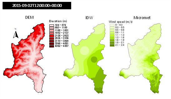
Fig. 2.19 Wind speed at 12:00 of 2015-09-02 on the Toce river, Italy, interpolated with inverse distance weighting without drift (moddle) and with elevation drift (right). Digital elevation model on the left.

BOX 2.D The Micromet method on the Upper Po river basin

Three spatial interpolation techniques – Thiessen, IDW, and Micromet – are evaluated on the upper Po river basin, in northern Italy. It covers 37200 km², of which 13700 km² (36.8%) have elevation higher than 1000 m (mountain), 10800 km² (29%) have elevation in the range 300 - 1000 m (hilly), and 12700 km2 (34.2%) lies below 300 m (flat).

The Upper Po river basin elevation model and wind gauging stations

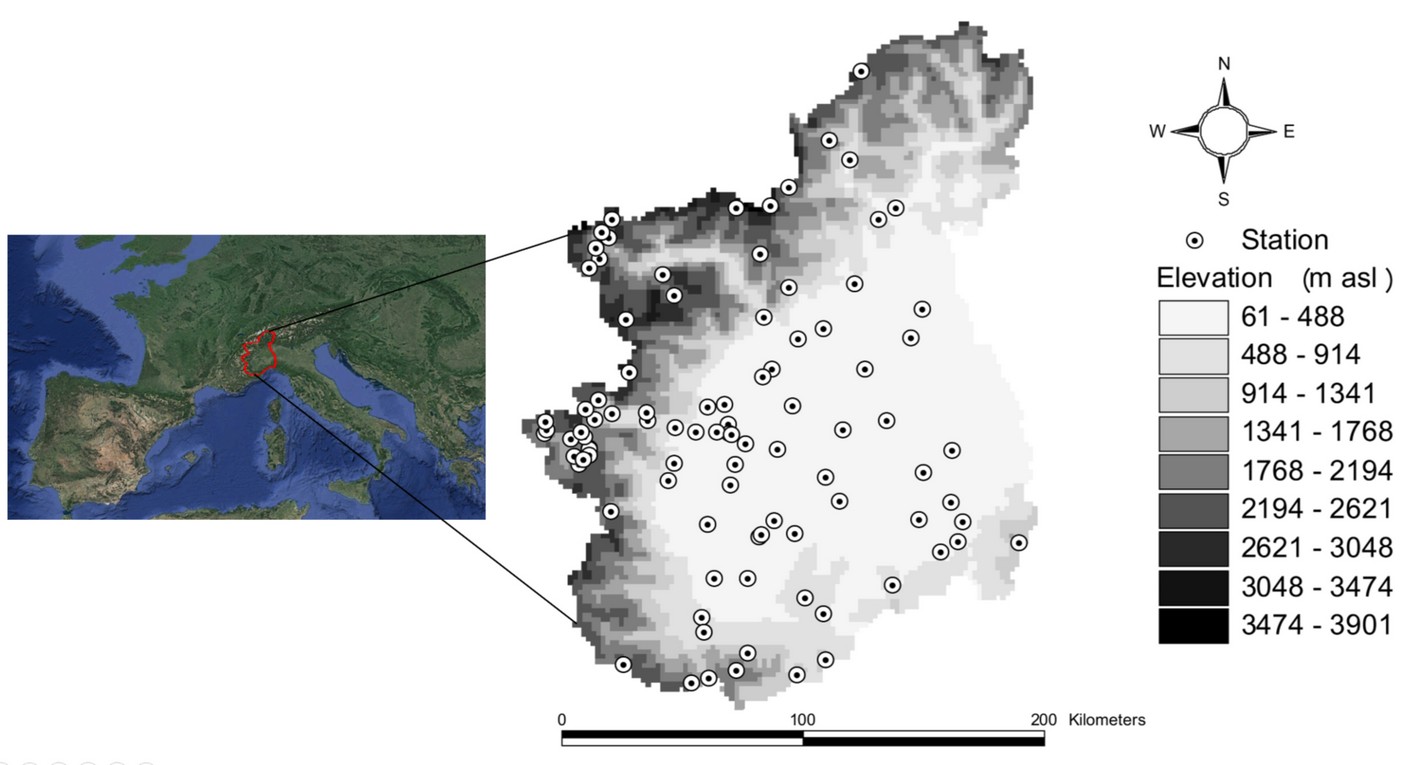
Performance of methods to interpolate wind speed data was assessed in terms of ability to reproduce the output of the MOLOCH meteorological model (Malguzzi et al., 2006), considered as the benchmark solution. To this purpose, for each of the first 24 hours of daily MOLOCH run, the \(u\) and \(v\) wind components of all cells that include one monitoring station, were extracted and converted to wind speed and direction This procedure allowed to reconstruct a continuous time series of virtual wind speed and direction data for the 95 stations over the Upper Po river basin. When Micromet method was applied, the same elevation model implemented in the MOLOCH model was used. Therefore, an interpolation method perfectly performing should reproduce exactly the MOLOCH output.

Performance results in terms of normalised root mean square error (NRMSE) and the relative bias (RB) computed on three elevation ranges.

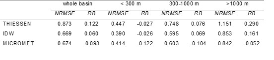
Results show that Micromet is able to increase the accuracy of wind speed interpolation only in the area where topography plays a relevant role (higher elevations). In other areas (as plain or hill), simple IDW is better than the other two methods. More details in Ravazzani et al., 2020.

2.5.2. The González-Longatt model

The orographic correction is used to modify the horizontal wind velocity components based on the elevation differences from the horizontally interpolated terrain elevations.

The orographic correction of both horizontal velocity components is determined by adding a correction calculated using the function \(f\) to the initially estimated velocity components \(u\) and \(v\), see equations (2.51) and (2.52), which result from the initial spatial interpolation of the measured wind speed datasets. The function \(f\) is consequently used in order to include a correction due to terrain orography and it can be justified based on both the conservation of mass and the conservation of momentum principles applied to a streamline (see Fig. 2.20 ) where an increase in height \(\Delta h\) requires also an increase in velocity. The conservation of mass indicates that as the density decreases, as it is the case in atmospheric flows where all the state variables decrease with increasing altitude, the velocity must increase in order to maintain mass flow constant. Alternatively, the form adopted for the function \(f\) can be justified based on the conservation of momentum equation where the term \(- \partial P/\partial x_{i}\) acts as a momentum sink if the pressure gradient increases in all spatial coordinates and as a source term if the pressure spatial gradient decreases as it is the case when the terrain altitude increases.

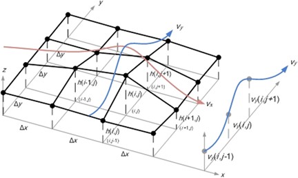
Fig. 2.20 Schematic showing the horizontal discretization around an arbitrary grid point \((i, j)\) at height \(h(i, j)\) whose velocity components \(V_{x}(i, j)\) and \(V_{y}(i, j)\) is calculated using the orographic correction. (source: González-Longatt et al. (2015))

However, for simplicity, the formulation of the function \(f\) assumes that pressure changes are linearly related to changes in height (\(\Delta h\)). Additionally, it is worth highlighting a favourable feature of the correction function \(f\), that is, it is inversely proportional to the grid spacing (\(\Delta x\)). This has the effect of reducing the level of correction introduced by Eqs. (2.60) and (2.61) as the grid resolution is decreased which serves to minimise potential errors in the corrected wind velocity components for grids with insufficient or low density.

(2.60)\[V_{x}^{calc} = \ V_{x} + f\left( \mathrm{\Delta}h\frac{\mathrm{\Delta}V_{x}}{\mathrm{\Delta}x} \right)\]

(2.61)\[V_{y}^{calc} = \ V_{y} + f\left( \mathrm{\Delta}h\frac{\mathrm{\Delta}V_{y}}{\mathrm{\Delta}y} \right)\]

Finally, the orographic correction is implemented using a central difference calculation (see Fig. 2.20 ) around the grid node for which the velocity is to be corrected and the corrected velocity components (\(V_{x}^{calc}\) and \(V_{y}^{calc}\)) are calculated using the equations

(2.62)\[\begin{split}V_{x}^{calc} = \ V_{x} + \frac{1}{2}\left\lbrack \frac{\begin{array}{r} \left( h(i,j) - h(i - 1,j) \right) \times \left( V_{x}(i - 1,j) - V_{x}(i,j) \right) + \\ \left( h(i + 1,j) - h(i,j) \right) \times \left( V_{x}(i,j) - V_{x}(i + 1,j) \right) \\ \end{array}}{\mathrm{\Delta}x} \right\rbrack\end{split}\]

(2.63)\[\begin{split}V_{y}^{calc} = \ V_{y} + \frac{1}{2}\left\lbrack \frac{\begin{array}{r} \left( h(i,j) - h(i,j - 1) \right) \times \left( V_{y}(i,j - 1) - V_{y}(i,j) \right) + \\ \left( h(i,j + 1) - h(i,j) \right) \times \left( V_{y}(i,j) - V_{y}(i,j + 1) \right) \\ \end{array}}{\mathrm{\Delta}y} \right\rbrack\end{split}\]

Wind vector components, \(V_{x}^{calc}\) and \(V_{y}^{calc}\) are composed to compute the final corrected wind speed value, \(\mathbf{W}\)

(2.64)\[\mathbf{W}\mathbf{=}\sqrt{\left( V_{x}^{calc} \right)^{\mathbf{2}}\mathbf{+}\left( V_{y}^{calc} \right)^{\mathbf{2}}}\]

2.6. Mixing methods

The usual method to interpolate station data relies on the same spatial interpolation method for the whole domain. As an option the FeST model implements a fully flexible system that allows to define zones of the simulation domain where different interpolation methods are applied.

Fig. 2.21 shows an example of interpolation of precipitation measurements on the Toce river basin, Italy, assigning two different zones with id values 1 and 2 that corresponds to Thiessen and IDW interpolation methods, respectively. Fig. 2.22 shows an example of spatial interpolation of wind speed data on the Toce river basin, Italy, using two methods: the IDW in zone with elevation lower than 2000 m a.s.l., and the Micromet method where elevation is greater than 2000 m a.s.l..

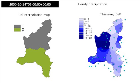
Fig. 2.21 Example of interpolation of precipitation measurements on the Toce river basin, Italy, assigning two different zones (left) with id values 1 and 2 that corresponds to Thiessen and IDW interpolation methods, respectively. Final interpolated map is shown on the right.

Fig. 2.22 Example of interpolation of wind speed data on the Toce river basin, Italy, using two methods: the IDW in zone with elevation lower than 2000 m a.s.l., and the Micromet method where elevation is greater than 2000 m a.s.l.. left map is obtained using only IDW, map in the middle is obtained using Micromet only, the right map is obtained with a mixing of the two methods.

2.7. Gridded meteorological data

When FeST is used for flood forecasting or climate change analysis purposes, the usual format of input data is multidimensional netCDF. Spatial reference system adopted by meteorological and climatic models that provide gridded datasets is usually geodetic (Fig. 2.23). Spatial resolution is usually coarser than hydrological simulation resolution. Gridded data are converted to the proper reference system and spatially downscaled to the simulation grid resolution with nearest neighbour resampling method (Fig. 2.24). This is a technique in which the value of each cell in an output raster is calculated using the value of the nearest cell in an input raster. Nearest neighbour assignment does not change any of the values of cells from the input layer. It preserves the original coarse grid structure, although the data is defined on a finer grid after resampling takes place.

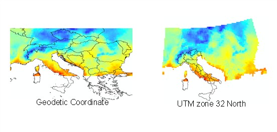
Fig. 2.23 Example of spatial reprojection of temperature data from geodetic reference system to UTM 32N.

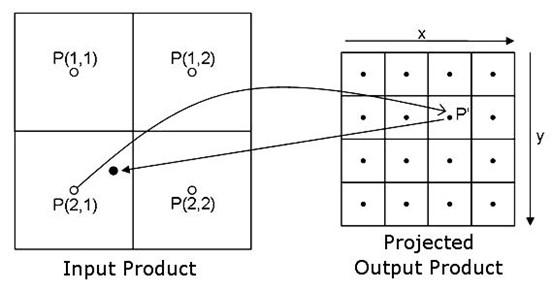
Fig. 2.24 Grid data resampling with nearest neighbour method. Source: https://www.brockmann-consult.de/beam/doc/help/general/ResamplingMethods.html